Air travel has become an integral part of modern life. In 2018, approximately 144 million people, which is nearly half of the American population, traveled on a plane and 15% of all domestic flights were delayed, according to data from the U.S. Department of Transportation. The motivation to build a Machine Learning model that best predicts departure delay is at high stakes for several reasons. Flight delays can cause inconvenience to passengers, result in missed connections, and even lead to financial losses for airlines. Our analysis is solely based on the year 2018 for American domestic flights, as it’s the most recent data that we can work with. During our work, we seek to predict the departure delay (DEP_DELAY), which is the subtraction between planned departure time (CRS_DEP_TIME) and the actual arrival time (DEP_TIME). In other words, we seek to predict if a given flight is going to depart late from its origin. According to the United States Federal Aviation Administration (FAA), a flight is delayed when it is 15 minutes later than its scheduled time. Therefore, we will consider a flight to be delayed at departure when the delay is equal or bigger than fifteen minutes.
Seasonality seems to be important when analyzing flight delays because the number of delays and their causes can vary depending on the time of year. Factors like weather conditions, holidays, and peak travel periods can all impact flight delays, making it important to account for seasonality in any analysis to gain a complete understanding of the data. Therefore, considering seasonality is crucial in analyzing flight delays as it allows for a comprehensive examination of the data by capturing the variations in delay occurrences and their underlying factors across different time periods
AIR_TIME: The time duration between wheels_off and wheels_on time (numerical).
DISTANCE: Distance between two airports (numerical).
CARRIER_DELAY: Delay caused by the airline in minutes (numerical).
WEATHER_DELAY: Delay caused by weather (numerical).
NAS_DELAY: Delay caused by air system (numerical).
SECURITY_DELAY: Delay caused by security (numerical).
LATE_AIRCRAFT_DELAY: Delay caused by security (numerical).
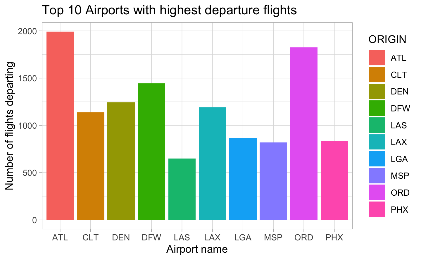
In order to address computational limitations, a subset of 12,000 observations was selected from a dataset comprising 7,213,446 flights. This subset was chosen to achieve a balanced representation of approximately one thousand flights per month. Subsequently, the subset was further filtered based on the top 10 airports with the highest number of departure flights, and a random selection of 50 destinations was made from the remaining flights.
A new variable called DELAY is introduced for classification tasks. It is defined as follows: if the computed difference between the planned departure time and actual arrival time (DEP_TIME - CRS_DEP_TIME) exceeds 15 minutes, indicating a delay in arrival, the value of the DELAY variable is assigned as 1. Conversely, if the computed difference is 15 minutes or less, indicating no or minimal delay, the value of the DELAY variable is set to 0.
Show the code
# Import the CSV fileairlines <-read.csv(here("data", "2018.csv"))# Filter the original data with the Top 10 airports with highest departure flightsairlines <- airlines %>%filter(ORIGIN %in%c("ATL", "CLT", "DEN", "DFW", "LAS", "LAX", "LGA", "MSP", "ORD", "PHX"))# We select 50 destinations at randomset.seed(123)selected_destinations <- airlines %>%distinct(DEST) %>%sample_n(min(50, n()))# Filter the original dataset with the destinationsairlines <- airlines %>%filter(DEST %in% selected_destinations$DEST)# Check the number of rows in the data frametotal_rows <-nrow(airlines)# Set the desired number of random observationsn <-12000# Randomly select the indices of the observationsset.seed(123)random_indices <-sample(1:total_rows, n)# Subset the dataframe using the random indicesairlines <- airlines[random_indices, ]# For classification purposes, we add a binary variable called DELAY. airlines$DELAY <-ifelse(airlines$DEP_DELAY >15, 1, 0)airlines$DELAY <-as.factor(airlines$DELAY)
Related Work
Nowadays, the demand for airline transportation is increasing significantly. Analysis of flight delay, therefore, has become a popular research area for machine learning. The report undertaken by Yuemin Tang [reference: https://dl.acm.org/doi/fullHtml/10.1145/3497701.3497725] has presented valuable insights in this domain.
Research questions
Our primary research objective revolves around the accurate prediction of flight departure delays using historical data from US flights in the year 2018. To accomplish this objective, we intend to employ the following classification models:
Supervised: Logistic Regression, Random Forest, K-Nearest Neighbors, Neural Networks and Support Vector Machines.
Unsupervised: Principal Component Analysis.
Secondly, given that a flight will be delayed on departure, we seek to quantify this delay, in minute intervals, using Linear regression and Support Vector Machines (multi-classification).
EDA
1 Distribution: histograms
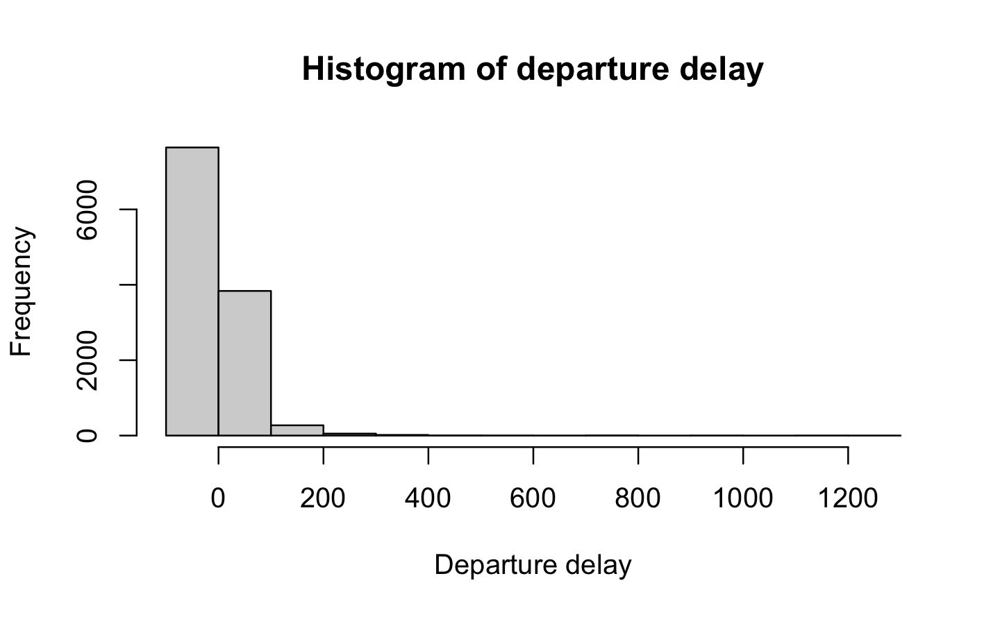
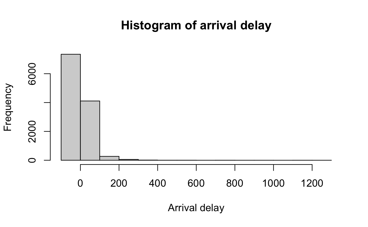
As stated in the first section, we observe that Arr_delay and Dep_delay are right-skewed - implying that the majority of domestic flights in the US in 2018 departed/arrived earlier than scheduled.
Show the code
hist(airlines$DEP_DELAY, main ="Histogram of departure delay", xlab ="Departure delay")hist(airlines$ARR_DELAY, main ="Histogram of arrival delay", xlab ="Arrival delay")
2 Delayed flights
Show the code
advance <-0advance0_15 <-0delay15_30 <-0delay30_45 <-0delay45_60 <-0delay60_plus <-0total <-0for (i in airlines$ARR_DELAY) {if (!is.na(i)) {if (i <0) { advance <- advance +1 } elseif (i <=15) { advance0_15 <- advance0_15 +1 } elseif (i <=30) { delay15_30 <- delay15_30 +1 } elseif (i <=45) { delay30_45 <- delay30_45 +1 } elseif (i <=60) { delay45_60 <- delay45_60 +1 } else { delay60_plus <- delay60_plus +1 } total <- total +1 }}# compute percentagespct_advance <- advance / total *100pct_advance0_15 <- advance0_15 / total *100pct_delay15_30 <- delay15_30 / total *100pct_delay30_45 <- delay30_45 / total *100pct_delay45_60 <- delay45_60 / total *100pct_delay60_plus <- delay60_plus / total *100tab <-matrix(c(pct_advance,pct_advance0_15 ,pct_delay15_30, pct_delay30_45, pct_delay45_60, pct_delay60_plus), ncol=6, byrow=TRUE)colnames(tab) <-c('Advance','Advance between 0 and 15 minutes','Delay between 15-30 minutes','Delay between 30-45 minutes','Delay between 45-60 minutes', 'Delay more than 60 minutes' )rownames(tab) <-"Percentage"tab <-as.table(tab)knitr::kable(tab)
Advance
Advance between 0 and 15 minutes
Delay between 15-30 minutes
Delay between 30-45 minutes
Delay between 45-60 minutes
Delay more than 60 minutes
Percentage
60.1
20.1
7.17
4.01
2.27
6.4
Fact
In 2018, only 20% of American domestic flights departed later than scheduled (late by more than 15 minutes)
3 Seasonality?
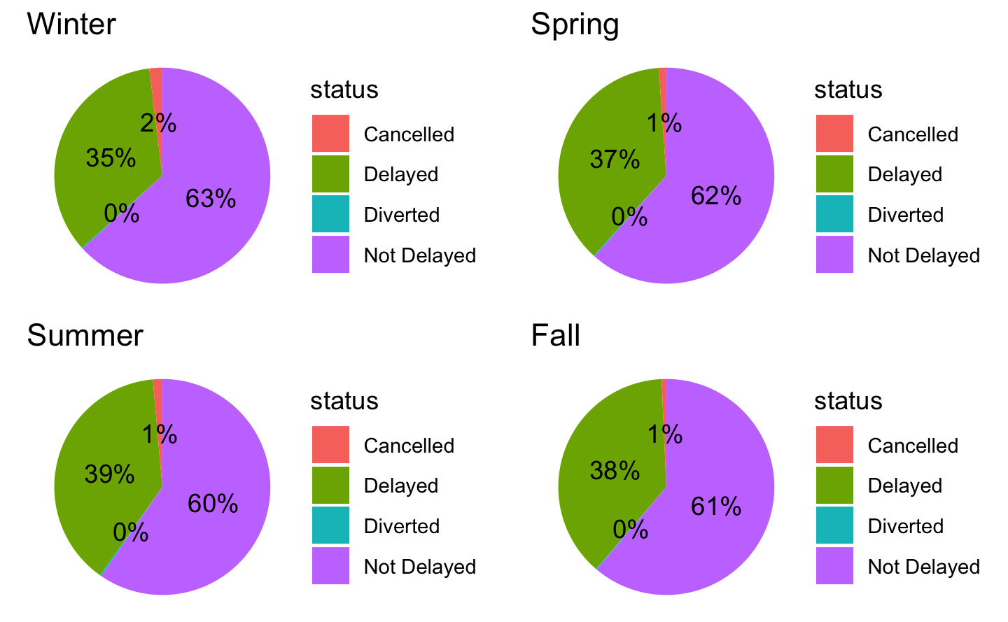
3.1 Proportion of delayed, diverted and cancelled flights across seasons
Our first intuition when analysing seasonality is that it does not seem to exist a significant difference of departure delay across seasons. As we can see, the biggest difference across seasons is between Summer and Winter.
Show the code
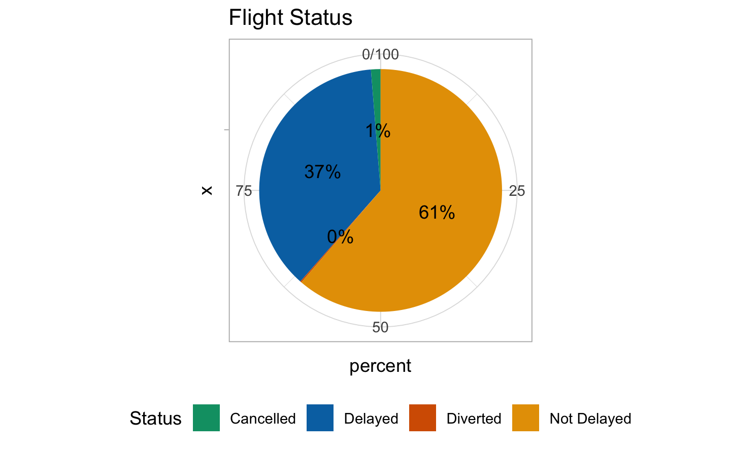
# Partition date into seasons (every 3 months)airlines$FL_DATE_NEW <-ymd(airlines$FL_DATE)airlines$season <-cut(month(airlines$FL_DATE_NEW), breaks=c(0,3,6,9,12), labels=c("Winter","Spring","Summer","Fall"))# Create a list to store the four pie chartspie_charts <-list()# Loop through the four seasons and create a pie chart for each# Loop through the four seasons and create a pie chart for eachfor (s inc("Winter", "Spring", "Summer", "Fall")) {# Filter the data for the current season season_data <- airlines %>%filter(season == s)# Check if the filtered data frame is emptyif (nrow(season_data) ==0) {# Skip to the next season if there are no flights in this seasonnext }# Compute the counts for each flight status delayed <-sum(season_data$ARR_DELAY >0, na.rm =TRUE) cancelled <-sum(season_data$CANCELLED ==1, na.rm =TRUE) diverted <-sum(season_data$DIVERTED ==1, na.rm =TRUE) not_delayed <-nrow(season_data) - delayed - cancelled - diverted# Create a data frame with the counts and labels flight_status <-data.frame(status =c("Delayed", "Cancelled", "Diverted", "Not Delayed"),count =c(delayed, cancelled, diverted, not_delayed))# Compute the percentages flight_status$percent <- flight_status$count /sum(flight_status$count) *100# Create the pie chart p <-ggplot(flight_status, aes(x ="", y = percent, fill = status)) +geom_bar(stat ="identity", width =1) +geom_text(aes(label =paste0(round(percent), "%")),position =position_stack(vjust =0.5)) +coord_polar("y", start =0) +theme_void() +ggtitle(s)# Add the pie chart to the list pie_charts[[s]] <- p}# Arrange the pie charts using grid.arrangegrid.arrange(grobs = pie_charts, ncol =2)# General pie chart delayed <-sum(airlines$ARR_DELAY >0, na.rm =TRUE)cancelled <-sum(airlines$CANCELLED ==1, na.rm =TRUE)diverted <-sum(airlines$DIVERTED ==1, na.rm =TRUE)not_delayed <-nrow(airlines) - delayed - cancelled - diverted# Create a data frame with the counts and labelsflight_status <-data.frame(status =c("Delayed", "Cancelled", "Diverted", "Not Delayed"),count =c(delayed, cancelled, diverted, not_delayed))# Compute the percentagesflight_status$percent <- flight_status$count /sum(flight_status$count) *100# Create the pie chartggplot(flight_status, aes(x ="", y = percent, fill = status)) +geom_bar(stat ="identity", width =1) +coord_polar("y", start=0) +labs(title ="Flight Status", fill ="Status") +theme(legend.position ="bottom") +geom_text(aes(label =paste0(round(percent), "%")), position =position_stack(vjust =0.5)) +scale_fill_manual(values =c("#009E73", "#0072B2", "#D55E00", "#E69F00"))
Fact
61% of flights are neither delayed, diverted or cancelled. 37% of flights are delayed. 2% of flights are cancelled. 0.28% are diverted.
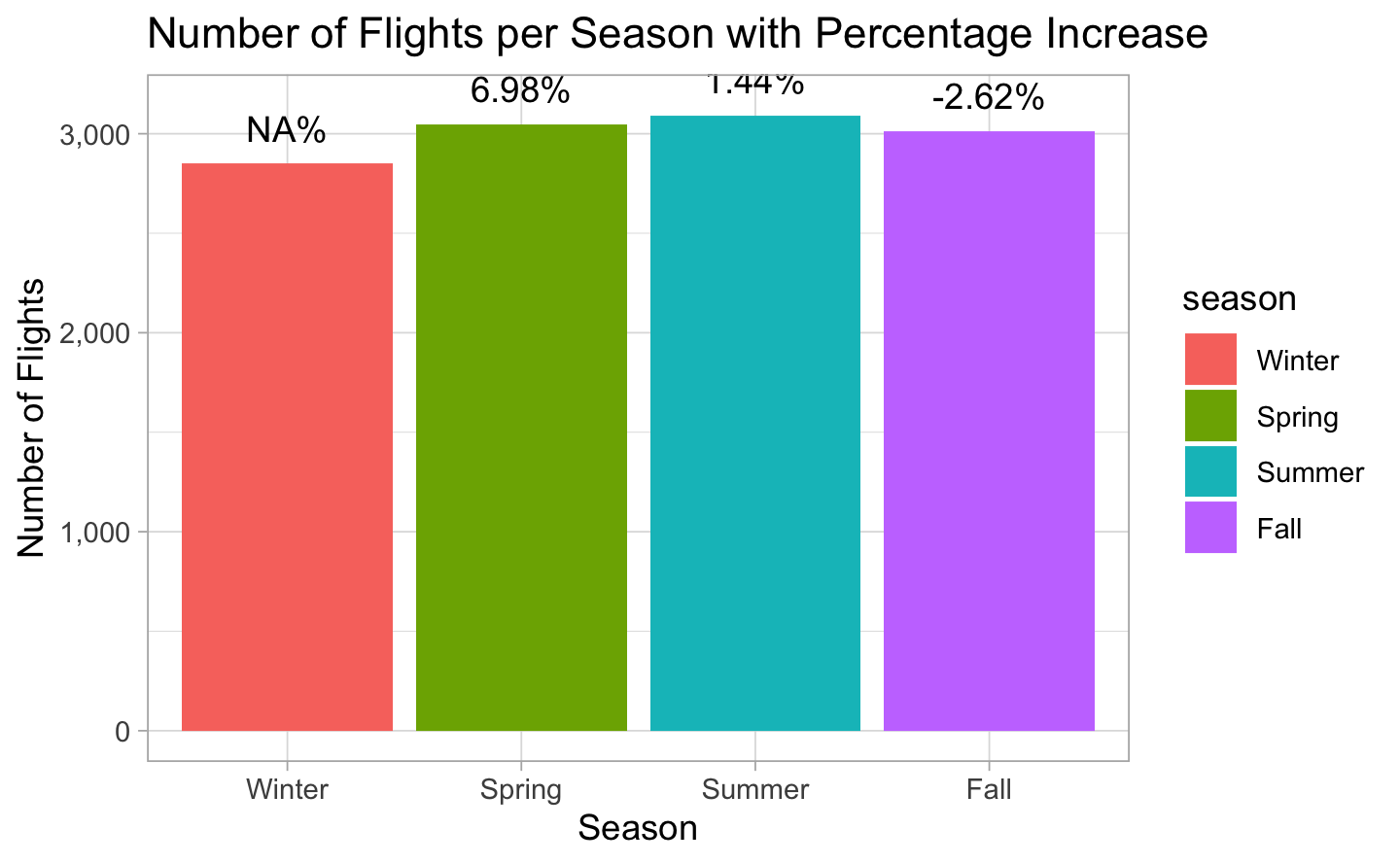
3.2 Number of flights
To investigate the presence of seasonality, we have created a variable called Season by partitioning the FL_DATE_NEW into 3-month intervals. The percentage change between consecutive seasons was computed by subtracting the current season’s flight count from the previous season’s flight count. However, the Winter season had a missing value due to the absence of a preceding season. Our analysis indicates that the number of flights fluctuates slightly across seasons, with the largest variation occurring between Winter and Summer, where the number of flights increased by 10%. This observation is consistent with the higher demand for flights during the summer vacation period. Further investigation is necessary to determine if seasonality is present in the data.
Show the code
# Compute the count of flights per seasonflights_count <- airlines %>%group_by(season) %>%summarise(count =n())# Compute the percentage increase in flights count between each seasonflights_count <- flights_count %>%mutate(percent_increase =round((count -lag(count)) /lag(count) *100, 2))# Create the bar plot with percentage increaseggplot(flights_count, aes(x = season, y = count, fill = season)) +geom_bar(stat ="identity") +geom_text(aes(label =paste0(percent_increase, "%"), y = count +50), vjust =-0.5) +labs(title ="Number of Flights per Season with Percentage Increase", x ="Season", y ="Number of Flights") +scale_y_continuous(labels = scales::comma)# Compute the percentage of evolution between Winter and Summer using the values in flights_countcat("The percentage increase of flight numbers from Winter to Summer is", round((flights_count$count[3] - flights_count$count[1]) / flights_count$count[1] *100, 2), "%")#> The percentage increase of flight numbers from Winter to Summer is 8.53 %
Fact
The percentage increase of flight numbers from Winter to Summer is around 8%
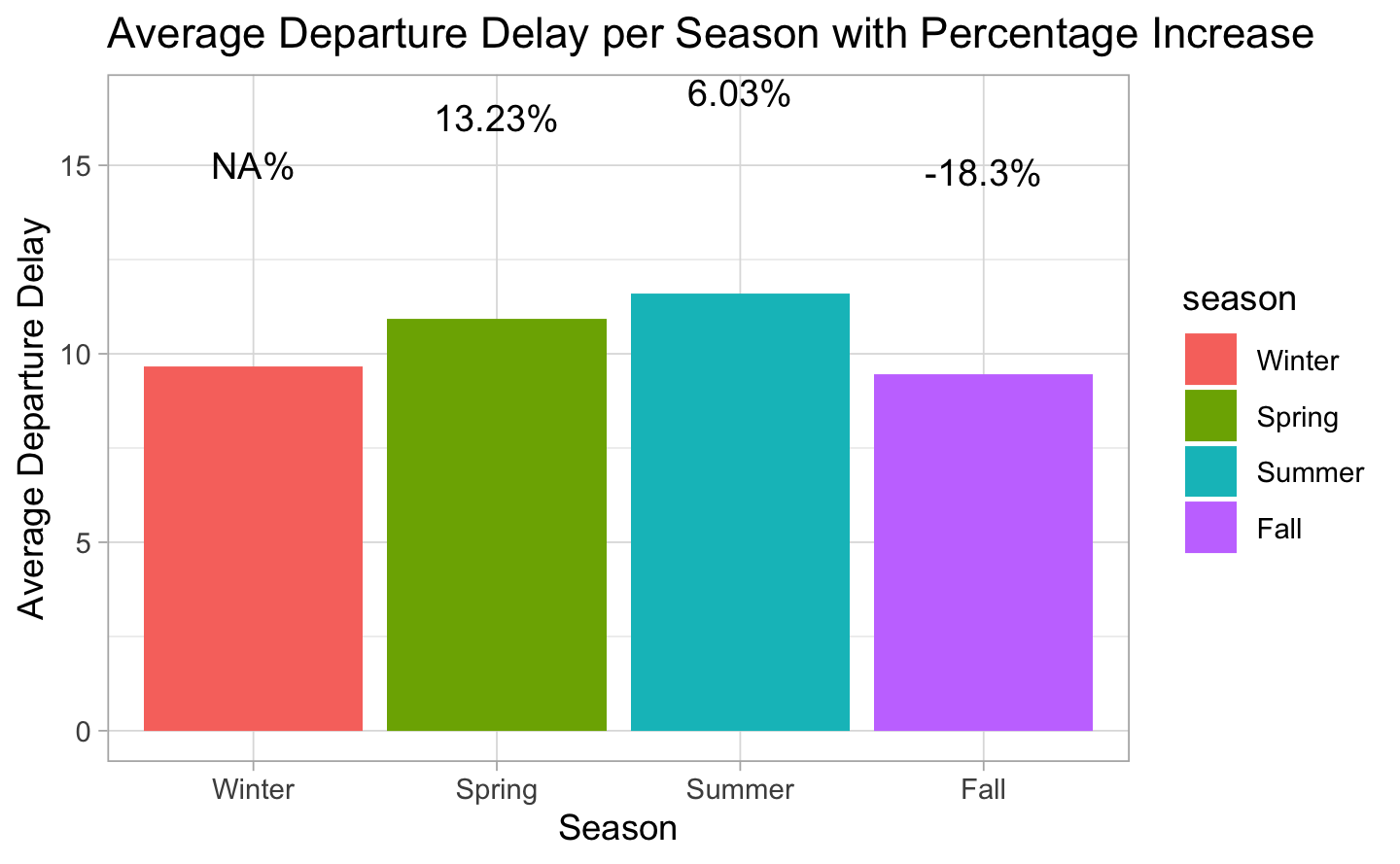
3.3 Response variable
Based on the observed bar plot, it can be deduced that the average departure delay is the highest during the Summer season as compared to the other seasons. Further analysis revealed a considerable 20.1% increase in the average arrival delay between the Winder and Summer seasons. Such a substantial difference in delay values could potentially create bias in our analysis and consequently, it is imperative to acknowledge and consider the impact of seasonality in our data set.
Show the code
# Compute the average delay per seasondelay_avg <- airlines %>%group_by(season) %>%summarize(avg_delay =mean(as.numeric(DEP_DELAY), na.rm =TRUE))# Compute the percentage increase in average delay between each seasondelay_avg <- delay_avg %>%mutate(percent_increase =round((avg_delay -lag(avg_delay)) /lag(avg_delay) *100, 2))# Create the bar plot with percentage increaseggplot(delay_avg, aes(x = season, y = avg_delay, fill = season)) +geom_bar(stat ="identity") +geom_text(aes(label =paste0(percent_increase, "%"), y = avg_delay +5), vjust =0, size =4) +labs(title ="Average Departure Delay per Season with Percentage Increase", x ="Season", y ="Average Departure Delay") +scale_y_continuous(labels = scales::comma)# Compute the percentage of evolution between Winter and Summer using the values in delay_avg cat("The percentage increase of average delay from Winter to Summer is", round((delay_avg$avg_delay[3] - delay_avg$avg_delay[1]) / delay_avg$avg_delay[1] *100, 2), "%")#> The percentage increase of average delay from Winter to Summer is 20.1 %
Fact
The percentage increase of average departed delay from Winter to Summer is of 20%
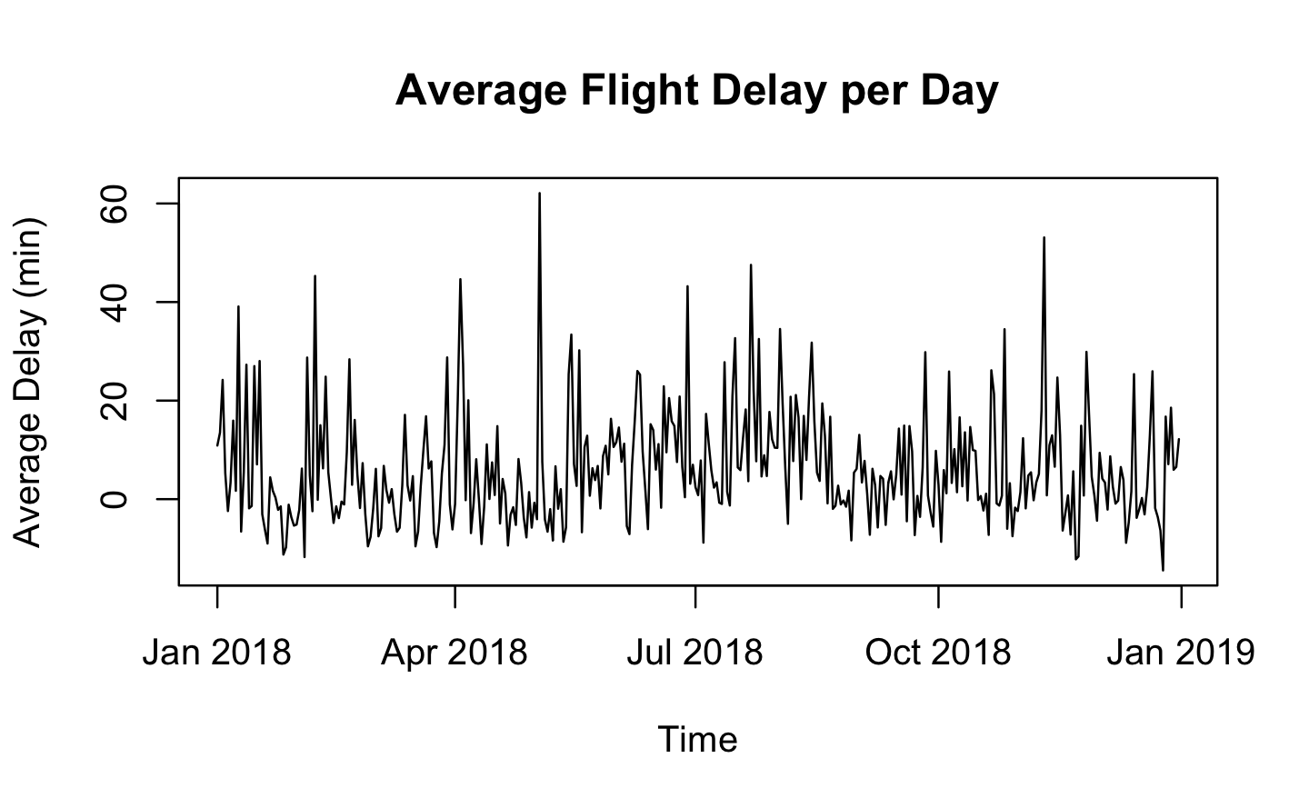
Undoubtedly, seasonality is a significant factor that needs to be taken into consideration as there are distinct patterns between seasons, which have the potential to cause bias in our analysis. Particularly in December, there are notable variations in the average departure delay. Thus, if we intend to forecast a flight delay, the season in which the flight operates significantly impacts the anticipated delay.
Show the code
# Remove rows with NA values in ARR_DELAY columnairlines_clean <- airlines[!is.na(airlines$ARR_DELAY),]# Convert ARR_DELAY column to numericairlines_clean$ARR_DELAY <-as.numeric(airlines_clean$ARR_DELAY)# Aggregate by FL_DATE_NEW and calculate mean ARR_DELAY for each groupairlines_avg <-aggregate(ARR_DELAY ~ FL_DATE_NEW, data = airlines_clean, FUN = mean)plot(airlines_avg$FL_DATE_NEW, airlines_avg$ARR_DELAY, type ="l", main ="Average Flight Delay per Day", xlab ="Time", ylab ="Average Delay (min)")
3.4 Total Delay Minutes by Delay Type across Seasons
In this section, we are going to investigate in depth the type of delay across seasons. As stated above, we observe that Summer has the highest number of delay types (larger number of delays in general). It’s important to point out that this is not the count, but the total sum of total delays in minutes. We observe that security_delay varies vastly among seasons, while carrier_delay is the most stable of all.
Show the code
# Only take observations which have a delaydelay_data <- airlines %>% dplyr::select(season, CARRIER_DELAY, WEATHER_DELAY, NAS_DELAY, SECURITY_DELAY, LATE_AIRCRAFT_DELAY) %>%pivot_longer(cols = CARRIER_DELAY:LATE_AIRCRAFT_DELAY, names_to ="delay_type", values_to ="delay_minutes") %>%filter(delay_type =="CARRIER_DELAY"& delay_minutes >0| delay_type =="WEATHER_DELAY"& delay_minutes >0| delay_type =="NAS_DELAY"& delay_minutes >0| delay_type =="SECURITY_DELAY"& delay_minutes >0| delay_type =="LATE_AIRCRAFT_DELAY"& delay_minutes >0) %>%group_by(season, delay_type) %>%summarise(total_delay_minutes =sum(delay_minutes, na.rm =TRUE))p <-ggplotly(ggplot(delay_data, aes(x = season, y = total_delay_minutes, fill = delay_type)) +geom_bar(stat ="identity") +labs(x ="Season", y ="Total Delay Minutes", fill ="Delay Type") +ggtitle("Total Delay Minutes by Delay Type and Season") +facet_wrap(~ delay_type, scales ="free_y"))p <-ggplotly(p, width =1500, height =300)p
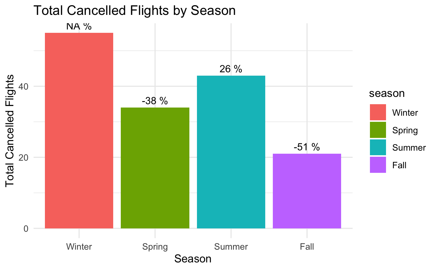
3.5 Cancellation and Diverted
Again, there is a huge variation between the seasons that confirms our seasonality assumption. Regarding cancellation, we observe that the higher variation across seasons is between Winter and Summer, with a decrease of more than 60%. This might occur because of harsher weather conditions during this period.
Show the code
cancelled_count <- airlines %>%group_by(season) %>%summarise(total_cancelled =sum(CANCELLED, na.rm =TRUE)) # only takes the values that are 1cancelled_count$percent_evolution <-c(NA, diff(cancelled_count$total_cancelled)/cancelled_count$total_cancelled[-length(cancelled_count$total_cancelled)]*100)ggplot(cancelled_count, aes(x=season, y=total_cancelled, fill=season)) +geom_bar(stat="identity") +labs(title="Total Cancelled Flights by Season",x="Season",y="Total Cancelled Flights") +geom_text(aes(label=paste(round(percent_evolution),"%")), vjust=-0.5, size=3.5) +theme_minimal()# Compute the percentage of evolution between Winter and Fall using the values in cancelled_countcat("The percentage decrease of cancelled fights from Winter to Fall is", round((cancelled_count$total_cancelled[4] - cancelled_count$total_cancelled[1]) / cancelled_count$total_cancelled[1] *100, 2), "%")#> The percentage decrease of cancelled fights from Winter to Fall is -61.8 %
Fact
The percentage decrease of cancelled fights from Winter to Fall is -61.8 %
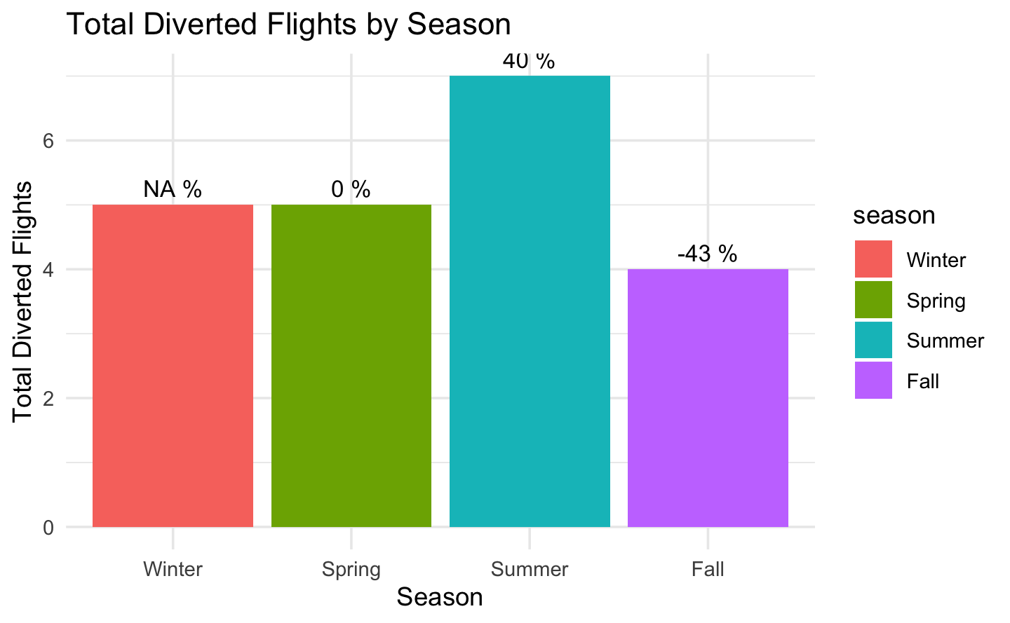
Regarding the diverted count, Summer has the highest number of planes diverted.
Show the code
diverted_count <- airlines %>%group_by(season) %>%summarise(total_diverted =sum(DIVERTED, na.rm =TRUE))diverted_count$percent_evolution <-c(NA, diff(diverted_count$total_diverted)/diverted_count$total_diverted[-length(diverted_count$total_diverted)]*100)ggplot(diverted_count, aes(x = season, y= total_diverted, fill = season))+geom_bar(stat ="identity")+labs(title="Total Diverted Flights by Season",x="Season",y="Total Diverted Flights") +geom_text(aes(label=paste(round(percent_evolution),"%")), vjust=-0.5, size=3.5) +theme_minimal()# Compute the percentage of evolution between Winter and Summer using the values in flights_count = 10%cat("The percentage increase of diverted flights from Winter to Summer is", round((diverted_count$total_diverted[3] - diverted_count$total_diverted[1]) / diverted_count$total_diverted[1] *100, 2), "%")#> The percentage increase of diverted flights from Winter to Summer is 40 %
Fact
The percentage increase of diverted flights from Winter to Summer is of 40%.
4 Exploring variables
4.1 Top 10 Airports with highest departures
Show the code
origin_count <- airlines %>%group_by(ORIGIN) %>%summarise(count =n()) %>%top_n(10, count) %>%arrange(desc(count))ggplot(origin_count, aes(x = ORIGIN, y = count, fill = ORIGIN)) +geom_bar(stat ="identity") +labs(title ="Top 10 Airports with highest departure flights", x ="Airport name", y ="Number of flights departing")
4.2 Top 10 airports with highest number of delayed flights
Show the code
# Calculate the count of delayed flights for each destination airportarrival_count <- airlines %>%filter(DEP_DELAY >0) %>%count(DEST, sort =TRUE) %>%rename(total_delayed = n) %>%top_n(10, total_delayed) %>%arrange(desc(total_delayed))# Filter and summarize data for top 10 airports with highest total delayed flightsarrival_data <- airlines %>%filter(DEST %in% arrival_count$DEST) %>%group_by(DEST) %>%summarise(avg_arr_delay =mean(as.numeric(ARR_DELAY), na.rm =TRUE),total_cancelled =sum(CANCELLED, na.rm =TRUE),total_diverted =sum(DIVERTED, na.rm =TRUE) ) %>%mutate(total_delayed = total_cancelled + total_diverted) %>%top_n(10, total_delayed) %>%arrange(desc(total_delayed))# Create first plot for average arrival delayplot1 <-plot_ly(arrival_data, x =~DEST, y =~avg_arr_delay, type ="scatter", mode ="markers",marker =list(color ="black", size =10),name ="Average Departure Delay") %>%layout(title ="Top 10 Airports with highest number of departure delayed flights",xaxis =list(title ="Airport name"),yaxis =list(title ="Average Arrival Delay"),width =800, height =600) # Adjust width and height as per your preference# Create second plot for sum of cancelled and diverted flightsplot2 <-plot_ly(arrival_data, x =~DEST, y =~total_cancelled, type ="bar", marker =list(color ="red"), name ="Cancelled Flights") %>%add_trace(y =~total_diverted, marker =list(color ="blue"), name ="Diverted Flights") %>%layout(xaxis =list(title ="Airport name"), yaxis =list(title ="Number of Flights"),barmode ="stack",width =800, height =600) # Adjust width and height as per your preference# Arrange the two plots side by sidesubplot(plot1, plot2, nrows =1)
Fact
The airport with the highest number of delayed and cancelled flights on departure is the Newark Liberty International Airport (EWR, New York).
4.3 Top 10 carriers with highest delays
Show the code
# Filter for flights with delayairlines_delay <- airlines %>%filter(!is.na(DEP_DELAY))# Calculate mean delay by carrier and sort in descending ordercarriers_delay <- airlines_delay %>%group_by(OP_CARRIER) %>%summarise(mean_delay =mean(DEP_DELAY, na.rm =TRUE)) %>%arrange(desc(mean_delay))# Get top 10 carriers with highest mean delaytop_10_carriers <-head(carriers_delay$OP_CARRIER, n =10)# Filter airlines_delay for top 10 carriersairlines_top <- airlines_delay %>%filter(OP_CARRIER %in% top_10_carriers)# Create plot with plotlyplot_top_carriers <-plot_ly(data = airlines_top, x =~OP_CARRIER, y =~ARR_DELAY, type ="box",boxpoints ="all", jitter =0.3, pointpos =-1.8,marker =list(color ="#FEE08B"),boxmean =TRUE) %>%layout(title ="Top 10 Carriers with Highest Departure Delays",xaxis =list(title ="Carrier", showgrid =FALSE, tickangle =45),yaxis =list(title ="Delay (minutes)", showgrid =TRUE),plot_bgcolor ="rgba(0,0,0,0)", paper_bgcolor ="rgba(0,0,0,0)",font =list(color ="#333333"),margin =list(b =0),boxmode ="group",showlegend =FALSE,width =800, height =800)# Update marker colorplot_top_carriers %>%layout(plot_bgcolor ="rgba(0,0,0,0)", paper_bgcolor ="rgba(0,0,0,0)",font =list(color ="#333333"),margin =list(b =0),boxmode ="group",showlegend =FALSE,marker =list(color =c("#FEE08B", "#FDAE61", "#F46D43", "#D53E4F", "#9E0142","#FEE08B", "#FDAE61", "#F46D43", "#D53E4F", "#9E0142")))
Show the code
# Remove the FL_DATE_NEW and Season Column
airlines <- dplyr::select(airlines, -FL_DATE_NEW, -season)
We can see that the carrier with the most frequent departure delay is United Airlines (UA). Meanwhile, the JetBlue Airways (B6) is far less likely to experience a departure delay.
5 Data
5.1 Describe Data
The initial analysis of our database involves the examination of the main structure using the str, summary and datatable functions.
Show the code
str(airlines)#> 'data.frame': 12000 obs. of 29 variables:#> $ FL_DATE : chr "2018-06-17" "2018-05-01" "2018-04-23"..#> $ OP_CARRIER : chr "UA" "DL" "F9" "9E" ...#> $ OP_CARRIER_FL_NUM : int 2133 2105 1188 3961 1413 2307 3513 245..#> $ ORIGIN : chr "LAS" "ATL" "PHX" "LGA" ...#> $ DEST : chr "EWR" "LIT" "CVG" "BUF" ...#> $ CRS_DEP_TIME : int 1404 1624 945 1930 2005 1410 1015 1025..#> $ DEP_TIME : num 1400 1628 941 1923 2004 ...#> $ DEP_DELAY : num -4 4 -4 -7 -1 1 -9 -5 2 -2 ...#> $ TAXI_OUT : num 19 13 13 33 11 13 12 79 12 12 ...#> $ WHEELS_OFF : num 1419 1641 954 1956 2015 ...#> $ WHEELS_ON : num 2133 1645 1611 2047 2020 ...#> $ TAXI_IN : num 7 4 8 5 5 8 6 8 4 17 ...#> $ CRS_ARR_TIME : int 2159 1659 1618 2109 2047 1522 1449 121..#> $ ARR_TIME : num 2140 1649 1619 2052 2025 ...#> $ ARR_DELAY : num -19 -10 1 -17 -22 -7 -35 58 -6 -23 ...#> $ CANCELLED : num 0 0 0 0 0 0 0 0 0 0 ...#> $ CANCELLATION_CODE : chr "" "" "" "" ...#> $ DIVERTED : num 0 0 0 0 0 0 0 0 0 0 ...#> $ CRS_ELAPSED_TIME : num 295 95 213 99 102 72 214 229 67 188 ...#> $ ACTUAL_ELAPSED_TIME: num 280 81 218 89 81 64 188 292 59 167 ...#> $ AIR_TIME : num 254 64 197 51 65 43 170 205 43 138 ...#> $ DISTANCE : num 2227 453 1569 292 453 ...#> $ CARRIER_DELAY : num NA NA NA NA NA NA NA 0 NA NA ...#> $ WEATHER_DELAY : num NA NA NA NA NA NA NA 0 NA NA ...#> $ NAS_DELAY : num NA NA NA NA NA NA NA 58 NA NA ...#> $ SECURITY_DELAY : num NA NA NA NA NA NA NA 0 NA NA ...#> $ LATE_AIRCRAFT_DELAY: num NA NA NA NA NA NA NA 0 NA NA ...#> $ Unnamed..27 : logi NA NA NA NA NA NA ...#> $ DELAY : Factor w/ 2 levels "0","1": 1 1 1 1 1 1 1 1..summary(airlines)#> FL_DATE OP_CARRIER OP_CARRIER_FL_NUM#> Length:12000 Length:12000 Min. : 3 #> Class :character Class :character 1st Qu.:1211 #> Mode :character Mode :character Median :2215 #> Mean :2619 #> 3rd Qu.:3739 #> Max. :7439 #> #> ORIGIN DEST CRS_DEP_TIME DEP_TIME #> Length:12000 Length:12000 Min. : 1 Min. : 1 #> Class :character Class :character 1st Qu.:1005 1st Qu.:1007 #> Mode :character Mode :character Median :1400 Median :1405 #> Mean :1406 Mean :1409 #> 3rd Qu.:1835 3rd Qu.:1843 #> Max. :2359 Max. :2400 #> NA's :150 #> DEP_DELAY TAXI_OUT WHEELS_OFF WHEELS_ON #> Min. : -49 Min. : 3.0 Min. : 1 Min. : 1 #> 1st Qu.: -5 1st Qu.: 13.0 1st Qu.:1026 1st Qu.:1139 #> Median : -2 Median : 17.0 Median :1422 Median :1541 #> Mean : 10 Mean : 19.4 Mean :1435 Mean :1522 #> 3rd Qu.: 7 3rd Qu.: 23.0 3rd Qu.:1900 3rd Qu.:2002 #> Max. :1238 Max. :146.0 Max. :2400 Max. :2400 #> NA's :162 NA's :152 NA's :152 NA's :154 #> TAXI_IN CRS_ARR_TIME ARR_TIME ARR_DELAY #> Min. : 1.0 Min. : 1 Min. : 1 Min. : -73 #> 1st Qu.: 4.0 1st Qu.:1155 1st Qu.:1138 1st Qu.: -13 #> Median : 5.0 Median :1555 Median :1541 Median : -5 #> Mean : 6.2 Mean :1546 Mean :1517 Mean : 6 #> 3rd Qu.: 7.0 3rd Qu.:2011 3rd Qu.:2002 3rd Qu.: 9 #> Max. :168.0 Max. :2359 Max. :2400 Max. :1231 #> NA's :154 NA's :154 NA's :183 #> CANCELLED CANCELLATION_CODE DIVERTED CRS_ELAPSED_TIME#> Min. :0.000 Length:12000 Min. :0.000 Min. : 44 #> 1st Qu.:0.000 Class :character 1st Qu.:0.000 1st Qu.: 90 #> Median :0.000 Mode :character Median :0.000 Median :126 #> Mean :0.013 Mean :0.002 Mean :140 #> 3rd Qu.:0.000 3rd Qu.:0.000 3rd Qu.:173 #> Max. :1.000 Max. :1.000 Max. :347 #> #> ACTUAL_ELAPSED_TIME AIR_TIME DISTANCE CARRIER_DELAY #> Min. : 37 Min. : 21 Min. : 108 Min. : 0 #> 1st Qu.: 85 1st Qu.: 62 1st Qu.: 425 1st Qu.: 0 #> Median :122 Median : 96 Median : 689 Median : 2 #> Mean :136 Mean :110 Mean : 806 Mean : 20 #> 3rd Qu.:170 3rd Qu.:142 3rd Qu.:1055 3rd Qu.: 20 #> Max. :388 Max. :341 Max. :2454 Max. :1231 #> NA's :174 NA's :174 NA's :9577 #> WEATHER_DELAY NAS_DELAY SECURITY_DELAY LATE_AIRCRAFT_DELAY#> Min. : 0 Min. : 0 Min. : 0 Min. : 0 #> 1st Qu.: 0 1st Qu.: 0 1st Qu.: 0 1st Qu.: 0 #> Median : 0 Median : 4 Median : 0 Median : 0 #> Mean : 4 Mean : 16 Mean : 0 Mean : 22 #> 3rd Qu.: 0 3rd Qu.: 20 3rd Qu.: 0 3rd Qu.: 26 #> Max. :726 Max. :984 Max. :126 Max. :686 #> NA's :9577 NA's :9577 NA's :9577 NA's :9577 #> Unnamed..27 DELAY #> Mode:logical 0 :9648 #> NA's:12000 1 :2190 #> NA's: 162 #> #> #> #> introduce(airlines)#> rows columns discrete_columns continuous_columns#> 1 12000 29 6 22#> all_missing_columns total_missing_values complete_rows#> 1 1 61656 0#> total_observations memory_usage#> 1 348000 2579200
Our data set contains 7,213,446 records of American domestic flights in 2018, with 28 variables in total. Of these variables, 22 are continuous, 5 are discrete, and 1 is missing (UNNAMED..27, which will be removed).
Let’s focus on both departure and arrival delays. On average, the departure delay is of 10 minutes and arrival delay is of 5 minutes. The median for departure is at -2 minutes, whereas at -6 minutes for arrival delay. This implies that the majority of American flights in 2018 departed and arrived earlier rather than late. Therefore, we expect the distribution to be right-skewed for both variables. We will explore more in depth the variables of interest after taking care of the missing values.
We can also observe that our data frame contains a lot of NA values in 16 of our variables. We will have to look into detail to see the reason why.
Furthermore, we have a lot of variables which describe a date or an hourly value, for example: ARR_TIME, WHEELS_ON, WHEELS_OFF and more. We need to convert them in order for our analysis to make sense.
Fact
The majority of domestic flights in the USA in 2018 either departed or arrived earlier than scheduled. Most delayed flight on arrival was of 45 hours!
5.2 Transform data
One crucial step in pre-processing our data set involves performing preliminary transformations, particularly converting several variables into a date, hour, or minute format. This conversion aims to represent the temporal aspects of the data more formally and facilitate subsequent analysis.
The only variable that needs to be converted to a full date format (year, month, day) is FL_DATE. We transform it using the Lubridate package.
We remove the Unnamed..27 variable which contains only NA values.
Show the code
airlines <- dplyr::select(airlines, -Unnamed..27)
Next, we deal with the variables having hour and minutes format. This corresponds to features such as DEP_TIME, WHEELS_OFF, ARR_TIME, where we consider a specific time during the day.
5.3 Dealing with missing values
Now, we can have a look at the missing values in our data set.
Show the code
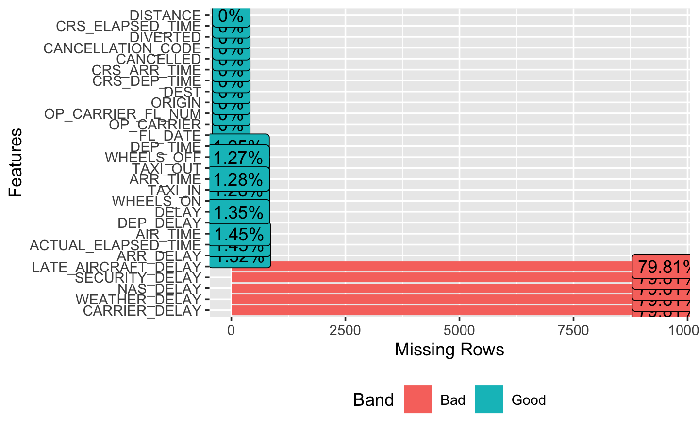
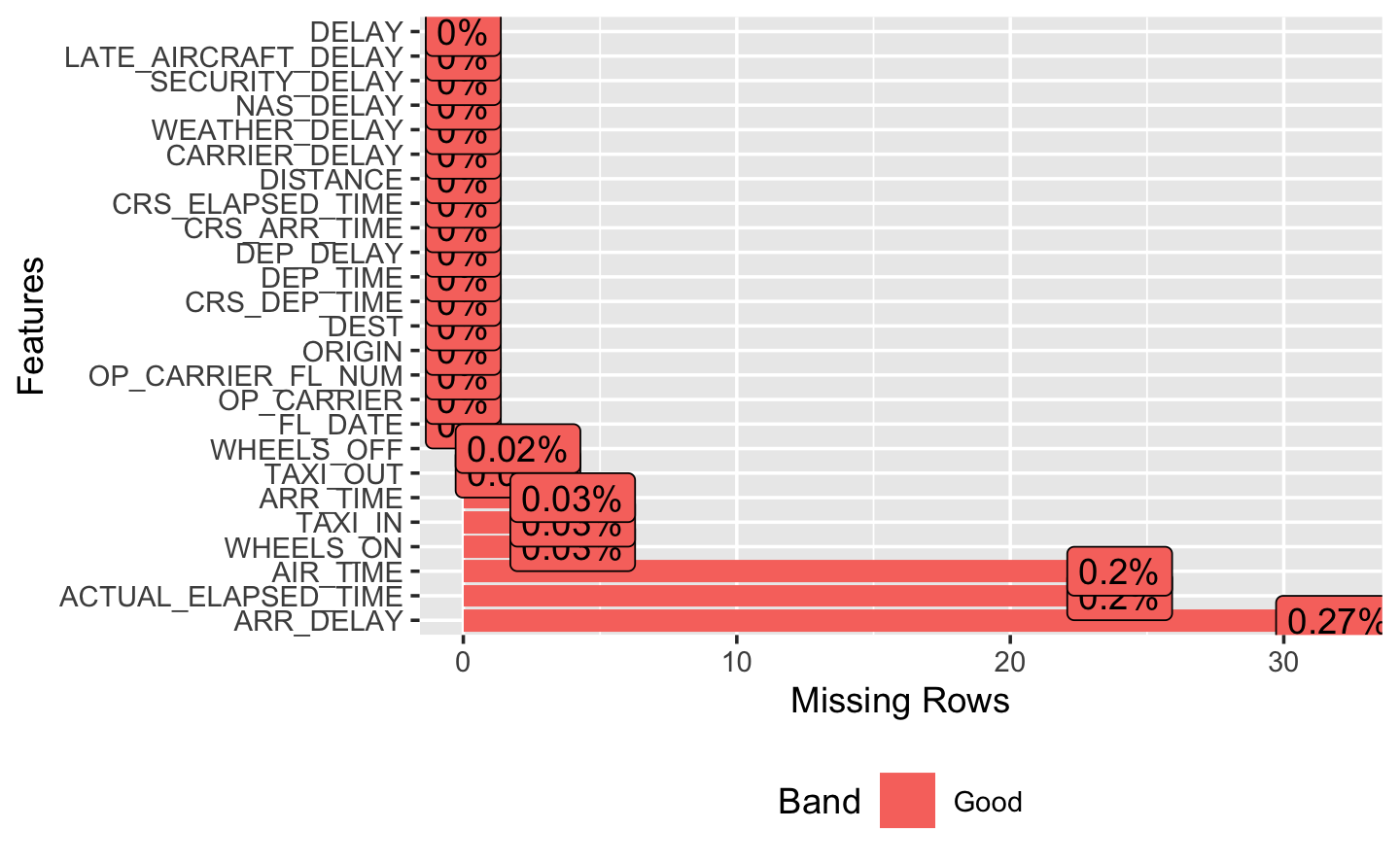
plot_missing(airlines) # check missing values
We see that we have approximately 80% of NA’s for 5 variables: CARRIER_DELAY, WEATHER_DELAY, NAS_DELAY, SECURITY_DELAY, LATE_AIRCRAFT_DELAY.
These missing values represent two things. First, it can indicate that the given flight had no delay. Or, if there was a delay, there would still be a NA value for flights that do not belong to that specific reason. Therefore, we will transform these missing values to 0.
Show the code
# Replace NA values with 0 in selected columnsairlines <- airlines %>%mutate(CARRIER_DELAY =ifelse(is.na(CARRIER_DELAY), 0, CARRIER_DELAY),WEATHER_DELAY =ifelse(is.na(WEATHER_DELAY), 0, WEATHER_DELAY),NAS_DELAY =ifelse(is.na(NAS_DELAY), 0, NAS_DELAY),SECURITY_DELAY =ifelse(is.na(SECURITY_DELAY), 0, SECURITY_DELAY),LATE_AIRCRAFT_DELAY =ifelse(is.na(LATE_AIRCRAFT_DELAY), 0, LATE_AIRCRAFT_DELAY) )
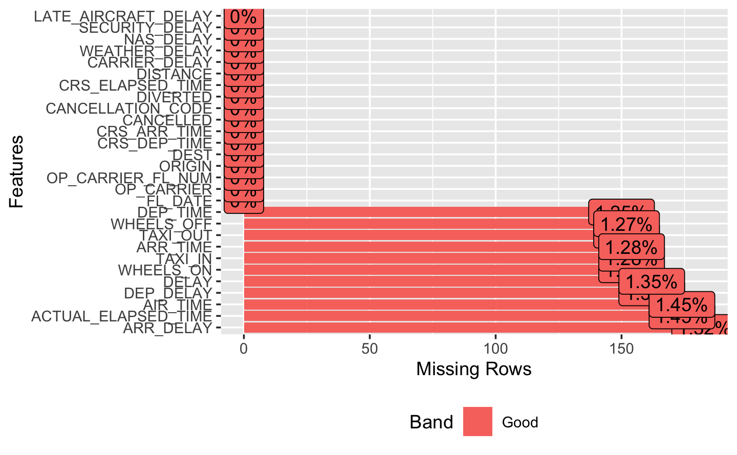
We plot again the missing values to check whether there have been improvements.
Show the code
plot_missing(airlines)
Indeed, the 5 variables we modified do not contain any NA’s.
Next, we have to take care of the last 10 variables. The range of missing values for all of these variables goes from ~ 1.6 to 2%. They seem to be somewhat connected between each other, just like the ones before. Since our variable of interest ARR_DELAY is part of them, we have to carefully look at their structure.
Let’s first explore our dataset containing only these NA’s.
FL_DATE
OP_CARRIER
OP_CARRIER_FL_NUM
ORIGIN
DEST
CRS_DEP_TIME
DEP_TIME
DEP_DELAY
TAXI_OUT
WHEELS_OFF
WHEELS_ON
TAXI_IN
CRS_ARR_TIME
ARR_TIME
ARR_DELAY
CANCELLED
CANCELLATION_CODE
DIVERTED
CRS_ELAPSED_TIME
ACTUAL_ELAPSED_TIME
AIR_TIME
DISTANCE
CARRIER_DELAY
WEATHER_DELAY
NAS_DELAY
SECURITY_DELAY
LATE_AIRCRAFT_DELAY
DELAY
2018-01-08
YX
4437
LGA
STL
1829
NA
NA
NA
NA
NA
NA
2030
NA
NA
1
B
0
181
NA
NA
888
0
0
0
0
0
NA
2018-01-05
9E
3355
LGA
RDU
630
NA
NA
NA
NA
NA
NA
823
NA
NA
1
C
0
113
NA
NA
431
0
0
0
0
0
NA
2018-02-05
MQ
3407
ORD
DSM
2035
NA
NA
NA
NA
NA
NA
2150
NA
NA
1
C
0
75
NA
NA
299
0
0
0
0
0
NA
2018-08-11
YV
5937
DFW
BMI
1250
NA
NA
NA
NA
NA
NA
1447
NA
NA
1
B
0
117
NA
NA
690
0
0
0
0
0
NA
2018-09-16
OH
5361
CLT
DAY
1140
NA
NA
NA
NA
NA
NA
1310
NA
NA
1
B
0
90
NA
NA
370
0
0
0
0
0
NA
Show the code
# Let's explore the NA's: we compute the % of cancellation flights to see if they correspond to the % of missing values of: DEP_TIME, DEP_DELAY, TAXI_OUT, WHEELS_OFF, WHEELS_ON, TAXI_IN, ARR_TIME, ARR_DELAY:freq <-table(airlines$CANCELLED)perc_1 <- freq[2] /length(airlines$CANCELLED) *100perc_0 <- freq[1] /length(airlines$CANCELLED) *100cat("Percentage of 1's:", round(perc_1, 2), "%\n")#> Percentage of 1's: 1.27 %cat("Percentage of 0's:", round(perc_0, 2), "%\n")#> Percentage of 0's: 98.7 %
As per their descriptions, the variables Taxi_out and Taxi_in are related to: Wheels_off, Wheels_on, Dep_time and Arr_time.
If a flight is cancelled, it means that the aircraft did not depart from the origin airport and did not arrive at the destination airport. Therefore, it is expected that variables related to departure and arrival times (such as Dep_time, Dep_delay, Taxi_out, Wheels_off, Wheels_on, Taxi_in, Arr_time, and Arr_delay) would be represented as NA’s for cancelled flights.
It is also noteworthy that some of the variables that are represented as NA’s for cancelled flights (specifically, Wheels_off and Taxi_out) account for approximately 1.65% of the total observations in the dataset. This indicates that a relatively small proportion of flights in the dataset were cancelled, and that missing values for Wheels_off and Taxi_out are likely indicators of cancelled flights.
We can notice that most of the Na’s in Taxi_out will be associated with a missing value in Taxi_in. This is true for all of the occurrences where there has been a delay.
When a flight has been diverted, we will only have values for Taxi_in, as the flight never reached it’s destination.
In rare cases, we have values for Dep_time and Dep_delay and an NA in Arr_delay due to a cancellation. In these cases, the flight seems to have been cancelled almost immediately after taking off.
The NA values for Arr_delay are due to one of 3 scenarios: 1) Cancellation 2) Diverted 3) The arrival time is the same as the planned arrival time (therefore, should be 0).
Finally, we can see that every time we have an NA for Air_time, we will also have one for Actual_elapsed_time. It makes sense as the latter is a formula containing the former.
To sum up, we can be confident that our NA values make sense. Transforming these 10 variables is not necessary, as they are not binary responses as the other 5 we changed. They are continuous representing minutes. Removing them would also not be a good idea, as they contain important information on the nature of the delay (cancellation, diverted).
5.4 Dealing with outliers
Now that we are clear on our missing values, we can focus on the potential outliers we have in our data set.
We use the summary function to see the extreme cases.
Show the code
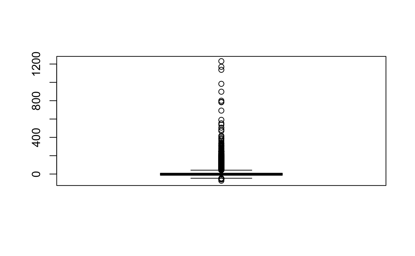
summary(airlines$ARR_DELAY)#> Min. 1st Qu. Median Mean 3rd Qu. Max. NA's #> -73 -13 -5 6 9 1231 183
We can note that our minimum and maximum values are respectively -2 hours and 20h 52 min. Both of these values are extreme.
Let’s visualize them using box plots.
Show the code
boxplot(airlines$ARR_DELAY)
We can see that we have a rather large spread of values, with some extreme cases going more than 1500 minutes. However, the mean and average are very close to zero, which is what we expected. Having such extreme cases doesn’t appear necessarily abnormal. Exceptional events such as extreme weather or other incidents can greatly impact the delay of air flights. We are going to keep these values during our modeling, as they represent event that, even though rare, are at risk of happening.
6 Data Transformations for the modelling part
6.1 Converting variables to factors
To apply Machine Learning models, such as Random Forest, we can’t have any numerical variable. Here, we transform them into factors.
Show the code
# We select columns that we will use to convert the integer to factormy_cols <-c(2, 4, 5, 16, 17, 18)# loop over each column and convert to factor in the bank datasetfor (i inseq_along(my_cols)) { airlines[[my_cols[i]]] <-factor(airlines[[my_cols[i]]])}
6.2 Classification: handling missing values
We have around 2% of missing values that represent the cancelled flights, therefore for each NA in DELAY we have decided to drop the instance. We removed 213 observations in airlines.
Show the code
airlines <- airlines[!is.na(airlines$DELAY), ]
6.3 Cancellation and Diverted
By removing the NA’s in DELAY, we eliminated all of the instances that represented a CANCELLATION. Furthermore, as our main analysis is about predicting flight delays and not cancelled flights neither diverted, we have decided to remove CANCELLED, CANCELLATION_CODE and DIVERTED from airlines and airlines_time. This enables us to have less variables in our data set.
The class distribution of our response variable is imbalanced. We found that approximately 80% of the observations belong to the “no-delay” class, while the remaining 20% belong to the “delay” class. The presence of class imbalance creates a situation where our models are more inclined to prioritize and predict the majority class (no-default) due to its higher prevalence in the data set. Consequently, this bias can result in sub-optimal performance when it comes to accurately identifying instances of the minority class (default), which is of particular importance in our analysis.
Moreover, the imbalanced class distribution leads to a distorted evaluation of model performance. Traditional evaluation metrics, such as accuracy, may be misleading and fail to capture the true predictive capabilities of the model. Machine learning algorithms that assume a balanced class distribution, such as Logistic regression, Support Vector Machines (SVM), and Neural Networks, may be particularly affected by this imbalance and yield compromised results.
Therefore, it is imperative for us to address the class imbalance issue in our modeling approach. During our class, we explored various methods to address class imbalance, including both up-sampling and down-sampling techniques. Among these methods, we found down-sampling to be our preferred approach as up-sampling can lead to the replication of existing observations or the introduction of unrealistic data points.
Show the code
class_distribution <-table(airlines$DELAY)percentage_0 <- class_distribution[1] /sum(class_distribution) *100percentage_1 <- class_distribution[2] /sum(class_distribution) *100print(paste("Percentage of 0's:", percentage_0))print(paste("Percentage of 1's:", percentage_1))
7.2 Metrics
In our analysis, our primary objective is to accurately predict the number of flights that will experience delays, which we consider as the positive class. Therefore, our focus will be on evaluating the sensitivity or recall metric, which measures the proportion of correctly predicted positive instances.
However, it’s important to note that when computing confusion matrices in R, the sensitivity value is often labeled as specificity, which can lead to confusion. To avoid this confusion, we will interpret the metric labeled as specificity as the sensitivity or recall in the context of our analysis.
Furthermore, since the distribution of delayed flights is imbalanced, with the majority of instances being non-delayed, we need to account for this imbalance. To address this, we will employ robust evaluation methods such as the F1-score and balanced accuracy.
By emphasizing the correct prediction of positive instances (delayed flights), we aim to prioritize the accurate identification of delays while maintaining a good overall balanced accuracy, which takes into account both the sensitivity and specificity of the model.
7.3 Methodology
For each model, we conducted a comparative analysis using Cross-Validation, Down-sampling and different data splitting techniques: fixed split, standard split, and rolling window cross-validation. These techniques enable us to partition the data set into training and testing subsets in distinct ways, allowing us to assess the model’s performance under different scenarios.
The fixed split technique ensures that the training data consists of observations with earlier dates, while the testing data comprises observations with later dates. This approach preserves the temporal order of the data in the split. By employing a fixed split, we create a training set that represents historical data and a testing set that simulates future, unseen data. This mimics the real-world scenario where we make predictions on future observations based on past information. Consequently, the model can learn and generalize from historical patterns, providing a more realistic evaluation of its performance on unseen data. In contrast, the standard split randomly assigns 80% of the data for training and 20% for testing, without considering the temporal relationship between observations. This can lead to poorer predictions since the random shuffling of data disrupts the temporal patterns.
Window cross-validation, on the other hand, involves iteratively training and testing the model using sliding windows of data. The window size determines the number of consecutive observations used for training, and the window step determines the interval between each window. This technique considers the temporal aspect by progressively moving the window through the data, ensuring that each observation is used for both training and testing. It provides a comprehensive evaluation of the model’s performance over time, capturing any changes or patterns in the data. For each of our model, we have tweaked the window size and step in order to optimize the results.
By comparing the results obtained from these different splitting techniques, we gain insights into how the model performs under various data partitioning strategies and can make informed decisions regarding the suitability of each approach for our specific modeling task.
Note
Due to computational limitations, we have been constrained to perform a maximum of five-fold cross-validation.
7.4 Splitting
We start by defining our default settings for partitioning the data into training and testing sets. In order to realistically simulate the scenario of a departure delay of a given day, we have decided to remove some variables to reduce bias. These variables are not known before the flight departure. For example, the real DEP_TIME and ARR_TIME. We only keep objective variables which are pre-defined (such as scheduled departure time).
Show the code
########### FIXED SPLIT ############### First step is to arrange the data from earliest to latest dateairlines <- airlines %>%arrange(FL_DATE)# Split_date using 80% for training and 20% testing; 80% of 12 is 9.6 so training from January until 18th of September. Testing between 19th of September until end of December. split_date <-as.Date("2018-09-18")# Split the datadf_tr_date <- airlines[airlines$FL_DATE < split_date, ]df_tr_date <- dplyr::select(df_tr_date, -DEP_TIME, -DEP_DELAY, -TAXI_IN, -TAXI_OUT, -WHEELS_OFF, -WHEELS_ON, -ARR_TIME, -ARR_DELAY, -ACTUAL_ELAPSED_TIME, -AIR_TIME, -NAS_DELAY, -WEATHER_DELAY,-CARRIER_DELAY,-SECURITY_DELAY, -LATE_AIRCRAFT_DELAY)df_te_date <- airlines[airlines$FL_DATE >= split_date, ]df_te_date <- dplyr::select(df_te_date, -DEP_TIME, -DEP_DELAY, -TAXI_IN, -TAXI_OUT, -WHEELS_OFF, -WHEELS_ON, -ARR_TIME, -ARR_DELAY, -ACTUAL_ELAPSED_TIME, -AIR_TIME, -NAS_DELAY, -WEATHER_DELAY,-CARRIER_DELAY,-SECURITY_DELAY, -LATE_AIRCRAFT_DELAY)########### RANDOM SPLIT ##############set.seed(123)trainIndex <-createDataPartition(airlines$DELAY, p =0.8, list =FALSE)df_tr <- airlines[trainIndex, ]df_tr <- dplyr::select(df_tr, -DEP_TIME, -DEP_DELAY, -TAXI_IN, -TAXI_OUT, -WHEELS_OFF, -WHEELS_ON, -ARR_TIME, -ARR_DELAY, -ACTUAL_ELAPSED_TIME, -AIR_TIME, -NAS_DELAY, -WEATHER_DELAY,-CARRIER_DELAY,-SECURITY_DELAY, -LATE_AIRCRAFT_DELAY)df_te <- airlines[-trainIndex, ]df_te <- dplyr::select(df_te, -DEP_TIME, -DEP_DELAY, -TAXI_IN, -TAXI_OUT, -WHEELS_OFF, -WHEELS_ON, -ARR_TIME, -ARR_DELAY, -ACTUAL_ELAPSED_TIME, -AIR_TIME, -NAS_DELAY, -WEATHER_DELAY,-CARRIER_DELAY,-SECURITY_DELAY, -LATE_AIRCRAFT_DELAY)########### WINDOW CROSS-VALIDATION ############### Best hyperparameters: # Define the window size and stepwindow_size <-1000# Set the window sizewindow_step <-500# Set the window step
7.5 Unsupervised
Principal Component Analysis
We need to manipulate date format to be able to use with PCA. Therefore, we extract and month and day components of FL_DATE.
Show the code
airlines2 <- airlines # Change the FL_DATE variable directlyairlines2$FL_DATE <-ymd(airlines2$FL_DATE)# Extract month and day from FL_DATEairlines2$Month <-month(airlines2$FL_DATE)airlines2$Day <-day(airlines2$FL_DATE)
Now, we are going to create a new data set which will contain the newly transformed variables, and we will apply one-hot encoding to each of them to have our data ready for our machine learning models.
Show the code
# Select the categorical variables to encodecat_vars <-c("OP_CARRIER","ORIGIN","DEST")# Perform one-hot encoding for each variable using lapply() and model.matrix()encoded_vars <-lapply(airlines2[cat_vars], function(x) model.matrix(~x-1, data = airlines2))# Rename the encoded columns with more informative namesfor (i inseq_along(cat_vars)) { var_name <- cat_vars[i] var_levels <-levels(airlines2[[var_name]]) col_names <-paste0(var_name, "_", var_levels)colnames(encoded_vars[[i]]) <- col_names}# Combine the encoded variables into a single data frame using cbind()airlines2 <-cbind(airlines, do.call(cbind, encoded_vars))# Remove the original columnsairlines2 <- airlines2 %>% dplyr::select(-c("OP_CARRIER","ORIGIN","DEST"))# Create a table for head(bank)table_head <-kable(head(airlines2), format ="html", row.names =FALSE) %>%kable_styling(full_width =FALSE, html_font ="Arial")# Print the tabletable_head
We fit our PCA model and plot the first 2 dimensions. At the same time, we can visualize the individual components of these dimensions.
Show the code
# Set the seed for reproducibilityset.seed(123)# Perform PCAairlines_pca <-PCA(airlines2[,], ncp =11 , graph =FALSE)# Visualize the variance explainedplot_var <-fviz_pca_var(airlines_pca)plot_var <-ggplotly(plot_var) %>%layout(width =800, height =600)# Visualize the PCA biplotplot_biplot <-fviz_pca_biplot(airlines_pca)plot_biplot <-ggplotly(plot_biplot) %>%layout(width =800, height =600)# Arrange the two plots side by sidesubplot(plot_var, plot_biplot, nrows =1)
Show the code
# Visualize the contributions to the first principal componentplot_contrib1 <-fviz_contrib(airlines_pca, choice ="var", axes =1)plot_contrib1 <-ggplotly(plot_contrib1) %>%layout(width =800, height =600)# Visualize the contributions to the second principal componentplot_contrib2 <-fviz_contrib(airlines_pca, choice ="var", axes =2)plot_contrib2 <-ggplotly(plot_contrib2) %>%layout(width =800, height =600)# Arrange the two plots side by sidesubplot(plot_contrib1, plot_contrib2, nrows =1)
Show the code
# Visualize the eigenvaluesplot_eig <-fviz_eig(airlines_pca, addlabels =TRUE, ncp =30)plot_eig <-ggplotly(plot_eig) %>%layout(width =800, height =600)# Display the interactive plotssubplot(plot_eig)
As we can see, the two most important dimensions, dimension 1 and dimension 2, explain a relatively low variance in our dataset, with 5.5% and 4.5% respectively. Some of the variables strongly associated with dimension 1 include DISTANCE, AIR_TIME, and CRS_ELAPSED_TIME. Similarly, dimension 2 is influenced by variables such as WHEELS_OFF, DEP_TIME, and CRS_DEP_TIME. While these variables seem to be related within their respective dimensions, it is challenging to conclude that they are individually relevant for predicting delays in our data set.
Supervised
RandomForest
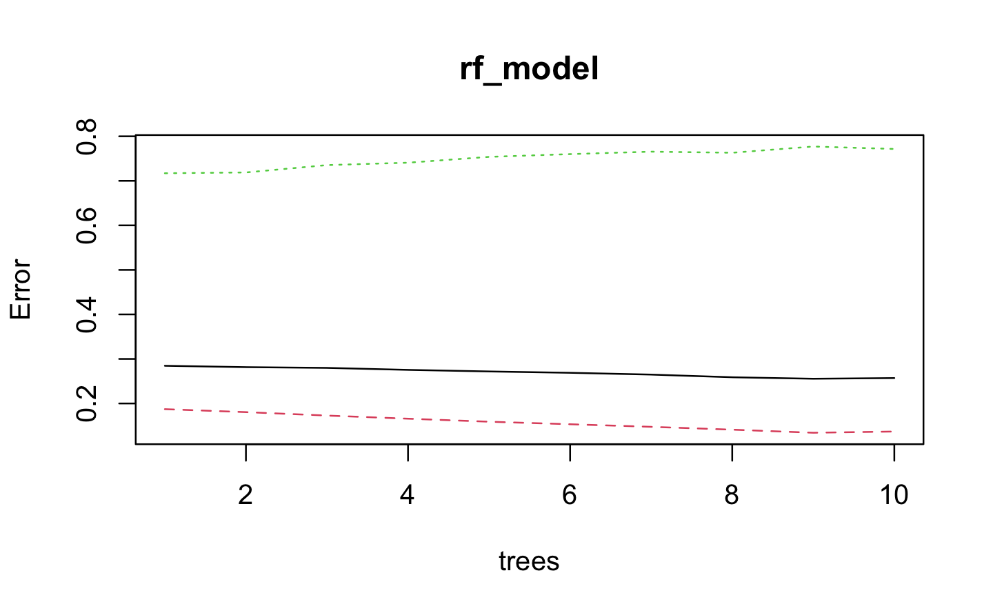
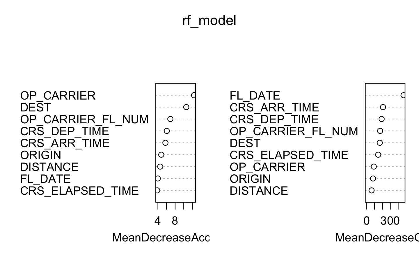
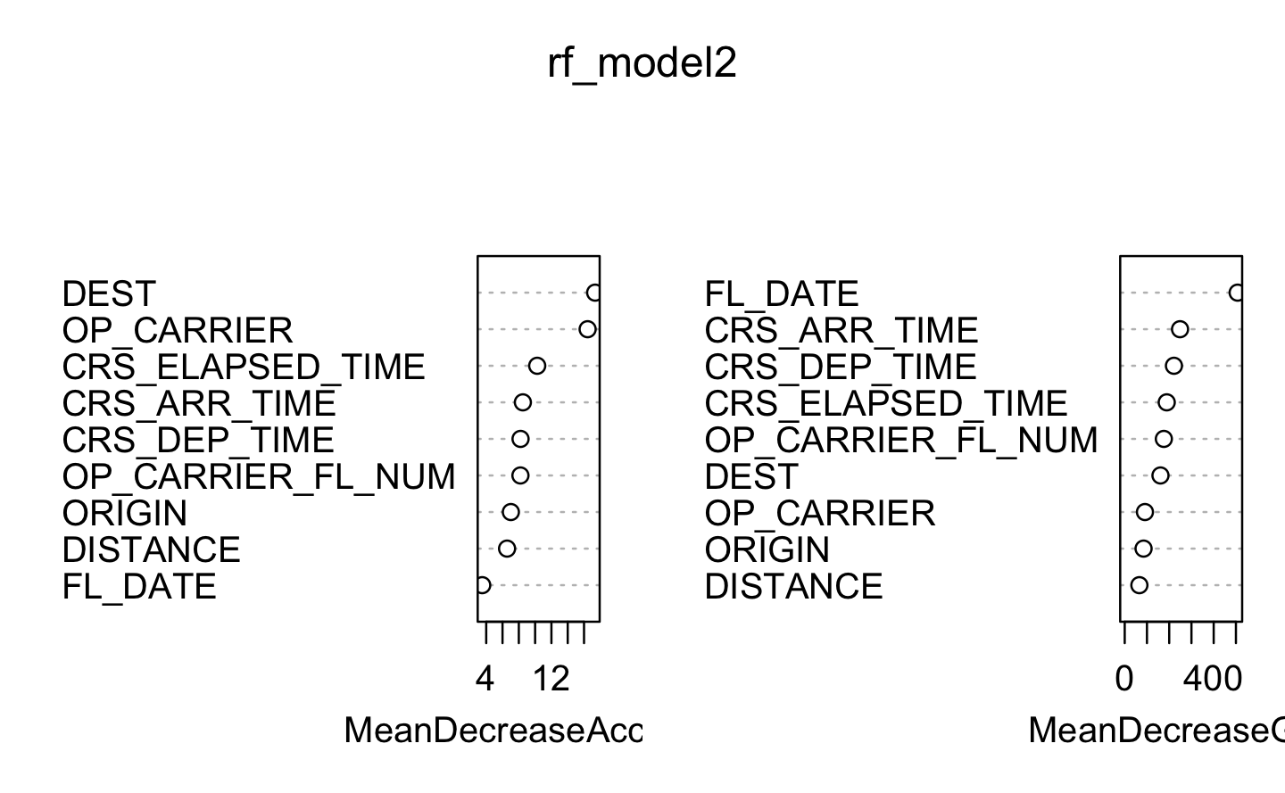
In randomForest, the variable importance is typically calculated based on the mean decrease in Gini index, as it tends to be more robust and interpretable than Mean Decrease Accuracy. randomForest function cannot handle a categorical predictor variable in a data set that has more than 53 categories. Using the sapply function we check that all the variables have less than or equal to 53 unique values. Due to computational limitations, we were unable to apply cross-validation in our analysis. The dataset used for training contains over 8000 observations, which makes the cross-validation method computationally expensive to implement along the random forest.
Show the code
########### 1. FIXED SPLIT: rf_model ############### Check that we have less or equal 53 unique values sapply(df_tr_date, function(x) length(unique(x))) # Use randomForest model set.seed(123)rf_model <-randomForest(DELAY ~ ., data = df_tr_date, ntree =10, mtry =5, importance =TRUE, localImp =TRUE, replace =FALSE, type ="classification")plot(rf_model)predictions <-predict(rf_model, newdata = df_te_date)confusionMatrix(predictions, df_te_date$DELAY) varImpPlot(rf_model, cex.axis =0.8)head(round(importance(rf_model), 2))########### 2. RANDOM SPLIT: rf_model2 ##############set.seed(123)rf_model2 <-randomForest(DELAY ~ ., data = df_tr, ntree =10, mtry =5, importance =TRUE, localImp =TRUE, replace =FALSE, type ="classification")predictions2 <-predict(rf_model2, newdata = df_te)confusionMatrix(predictions2, df_te$DELAY) varImpPlot(rf_model2, cex.axis =0.8)head(round(importance(rf_model2), 2))########### 3. WINDOW CV: rf_model3 ################# UNBALANCED #### Initialize variables to store the best confusion matrix and its performance measurebest_balanced_accuracy <-0best_confusion_matrix <-NULL# Perform window cross-validationset.seed(123)for (i inseq(1, nrow(df_tr_date), by = window_step)) {# Define the start and end indices of the current window start_index <- i end_index <-min(i + window_size -1, nrow(df_tr_date))# Extract the current window of data window_data <- df_tr_date[start_index:end_index, ]# Train the random forest model using the current window of data model <-train( DELAY ~ .,data = window_data,method ="rf",trControl =trainControl(method ="none"),tuneLength =1 )# Make predictions on the testing set predictions <-predict(model, newdata = df_te_date)# Compute the confusion matrix confusion_matrix <- caret::confusionMatrix(predictions, df_te_date$DELAY)# Calculate balanced accuracy balanced_accuracy <-mean(confusion_matrix$byClass[c("Sensitivity", "Specificity")])# Check if the current balanced accuracy is betterif (balanced_accuracy > best_balanced_accuracy) { best_confusion_matrix <- confusion_matrix best_balanced_accuracy <- balanced_accuracy }}# Print the best confusion matrix and balanced accuracycat("Best Confusion Matrix without balancing:\n")print(best_confusion_matrix)cat("Best Balanced Accuracy:", best_balanced_accuracy, "\n") ### BALANCED #### Initialize variables to store the best confusion matrix and its performance measurebest_balanced_accuracy <-0best_confusion_matrix <-NULL# Perform window cross-validationset.seed(123)for (i inseq(1, nrow(df_tr_date), by = window_step)) {# Define the start and end indices of the current window start_index <- i end_index <-min(i + window_size -1, nrow(df_tr_date))# Extract the current window of data window_data <- df_tr_date[start_index:end_index, ]# Perform down sampling on the current window of data downsampled_data <-downSample(x = window_data[, -which(names(window_data) =="DELAY")], y = window_data$DELAY)# Replace the name "Class" with "DELAY" in the downsampled datanames(downsampled_data)[names(downsampled_data) =="Class"] <-"DELAY"# Train the random forest model using the downsampled data model <-train( DELAY ~ .,data = downsampled_data,method ="rf",trControl =trainControl(method ="none"),tuneLength =1 )# Make predictions on the testing set predictions <-predict(model, newdata = df_te_date)# Compute the confusion matrix confusion_matrix <- caret::confusionMatrix(predictions, df_te_date$DELAY)# Calculate balanced accuracy balanced_accuracy <-mean(confusion_matrix$byClass[c("Sensitivity", "Specificity")])# Check if the current balanced accuracy is betterif (balanced_accuracy > best_balanced_accuracy) { best_confusion_matrix <- confusion_matrix best_balanced_accuracy <- balanced_accuracy }}# Print the best confusion matrix and balanced accuracycat("Best Confusion Matrix with balanced data:\n")print(best_confusion_matrix)cat("Best Balanced Accuracy:", best_balanced_accuracy, "\n")
Sensitivity
Specificity
F1-Score
Balanced Accuracy
Fixed Split - Unbalanced
17.3%
91.7%
22.0%
54.5%
Random Split - Unbalanced
17.4%
90.2%
18.6%
53.8%
Window CV (fixed split) - Unbalanced
22.7%
87.0%
21.7%
54.9%
Window CV (fixed split) - Balanced
62.7%
55.2%
33.6%
58.9%
In order to determine if a flight is going to be delayed upon departure by 15 minutes or more, the most important variables are: Flight date, Scheduled Arrival, Departure Time and Destination.
The most optimal model uses the window cross-validation split with downsampling. This makes sense as with this technique captures the hidden patterns in the data by taking into account temporality.
Fact
The Random Forest model that performs better is the window cross-validation when delay is balanced, with a sensitivity of 62.7% and balanced accuracy of 58.9%.
Logistic regression
This is a popular and intuitive model as it computes a probability for each observation to predict which class it should belong to.
Show the code
########### 1. FIXED SPLIT ##############set.seed(123)log_reg_model1 <-train( DELAY ~ .,data = df_tr_date,method ="glm",family ="binomial",trControl =trainControl(method ="cv", number =10))log_reg_model1balanced <-train( DELAY ~ .,data = df_tr_date,method ="glm",family ="binomial",trControl =trainControl(method ="cv", number =10, sampling ="down"))summary(log_reg_model1)summary(log_reg_model1balanced)predictions1 <-predict(log_reg_model1, newdata = df_te_date)predictions1balanced <-predict(log_reg_model1balanced, newdata = df_te_date)confusionMatrix(predictions1, df_te_date$DELAY) confusionMatrix(predictions1balanced, df_te_date$DELAY) ########### 2. SPLIT NORMAL: log_reg_model2 ##############set.seed(123)log_reg_model2 <-train( DELAY ~ .,data = df_tr,method ="glm",family ="binomial",trControl =trainControl(method ="cv", number =10))set.seed(123)log_reg_model2balanced <-train( DELAY ~ .,data = df_tr,method ="glm",family ="binomial",trControl =trainControl(method ="cv", number =10, sampling ="down"))summary(log_reg_model2)summary(log_reg_model2balanced)predictions2 <-predict(log_reg_model2, newdata = df_te)predictions2balanced <-predict(log_reg_model2balanced, newdata = df_te)confusionMatrix(predictions2, df_te$DELAY)confusionMatrix(predictions2balanced, df_te$DELAY) ########### 3. WINDOW CV: log_reg_model3: window uses fixed data split that takes into account temporality ################# UNBALANCED #### Define the window size and stepwindow_size <-2000# Set the window sizewindow_step <-1000# Set the window stepbest_balanced_accuracy <-0best_confusion_matrix <-NULLset.seed(123)# Perform window cross-validationfor (i inseq(1, nrow(df_tr_date), by = window_step)) {# Define the start and end indices of the current window start_index <- i end_index <-min(i + window_size -1, nrow(df_tr_date))# Extract the current window of data window_data <- df_tr_date[start_index:end_index, ]# Train the logistic regression model using the current window of data model <-train( DELAY ~ .,data = window_data,method ="glm",family ="binomial" )# Make predictions on the testing set predictions <-predict(model, newdata = df_te_date)# Compute the confusion matrix confusion_matrix <- caret::confusionMatrix(predictions, df_te_date$DELAY)# Calculate balanced accuracy balanced_accuracy <-mean(confusion_matrix$byClass[c("Sensitivity", "Specificity")])# Check if the current balanced accuracy is betterif (balanced_accuracy > best_balanced_accuracy) { best_confusion_matrix <- confusion_matrix best_balanced_accuracy <- balanced_accuracy }}# Print the best confusion matrix and balanced accuracycat("Best Confusion Matrix without balancing:\n")print(best_confusion_matrix)cat("Best Balanced Accuracy:", best_balanced_accuracy, "\n")### BALANCED ###best_balanced_accuracy <-0best_confusion_matrix <-NULLset.seed(123)# Perform window cross-validationfor (i inseq(1, nrow(df_tr_date), by = window_step)) {# Define the start and end indices of the current window start_index <- i end_index <-min(i + window_size -1, nrow(df_tr_date))# Extract the current window of data window_data <- df_tr_date[start_index:end_index, ]# Perform downsampling on the current window of data downsampled_data <- caret::downSample(x = window_data[, -which(names(window_data) =="DELAY")], y = window_data$DELAY)# Replace the name "Class" with "DELAY" in the downsampled datanames(downsampled_data)[names(downsampled_data) =="Class"] <-"DELAY"# Train the logistic regression model using the downsampled data model <-train( DELAY ~ .,data = downsampled_data,method ="glm",family ="binomial" )# Make predictions on the testing set predictions <-predict(model, newdata = df_te_date)# Compute the confusion matrix confusion_matrix <- caret::confusionMatrix(predictions, df_te_date$DELAY)# Calculate balanced accuracy balanced_accuracy <-mean(confusion_matrix$byClass[c("Sensitivity", "Specificity")])# Check if the current balanced accuracy is betterif (balanced_accuracy > best_balanced_accuracy) { best_confusion_matrix <- confusion_matrix best_balanced_accuracy <- balanced_accuracy }}# Print the best confusion matrix and balanced accuracycat("Best Confusion Matrix with balanced data:\n")print(best_confusion_matrix)cat("Best Balanced Accuracy:", best_balanced_accuracy, "\n")
Sensitivity
Specificity
F1-Score
Balanced Accuracy
Fixed Split - Unbalanced
4.3%
98.3%
6.5%
51.3%
Fixed Split - Balanced
71.9%
43.5%
32.6%
57.7%
Random Split - Unbalanced
0.4%
99.8%
2.3%
50.1%
Random Split - Balanced
61.4%
58.5%
35.7%
60.0%
Window CV (fixed split) - Unbalanced
64.9%
53.3%
33.5%
59.1%
Window CV (fixed split) - Balanced
86.7%
25.1%
31.9%
55.9%
Although the window cross-validation (balanced) has a good sensitivity, we are not going to select this one as the specificity is too low, implying that of all the flights that are not delayed, it would only correctly identify as non-delay 25%.
Surprisingly, the best model is the random split (balanced), even though it does not take temporality into account.
Tip
The Logistic Regression model that performs better is the random split when delay is balanced, with a sensitivity of 61.4% and balanced accuracy of 60%.
SVM
SVM method with the Radial Basis
Support Vector Machines (SVM) with a radial kernel are advantageous for classifying flight delays due to their ability to capture non-linear relationships between input features and the target variable. It can handle high-dimensional spaces, outliers and imbalanced data effectively, leading to accurate and robust predictions. Standardizing the data before SVM is necessary to ensure that all features contribute equally to the decision-making process, as SVM is sensitive to the scale of the features and may prioritize features with larger magnitudes. As we have mostly categorical variables, we couldn’t apply a standardization method. However, we tried using one-hot encoding to find an alternative solution. Unfortunately, the results were not congruent.
Show the code
########### 1. FIXED SPLIT: svm_model ##############set.seed(123)svm_model <-train( DELAY ~ .,data = df_tr_date,method ="svmRadial",trControl =trainControl(method ="cv", number =5),tuneLength =10)set.seed(123)svm_model_balanced <-train( DELAY ~ .,data = df_tr_date,method ="svmRadial",trControl =trainControl(method ="cv", number =5, sampling ="down"),tuneLength =10)# Print the model detailsprint(svm_model)print(svm_model_balanced)# Predict using the trained SVM modelpredictions <-predict(svm_model, newdata = df_te_date)predictions2 <-predict(svm_model_balanced, newdata = df_te_date)# Print the confusion matrix (for classification) confusionMatrix(predictions, df_te_date$DELAY) confusionMatrix(predictions2, df_te_date$DELAY) ########### 2. RANDOM SPLIT: svm_model_2 ##############set.seed(123)svm_model_2 <-train( DELAY ~ .,data = df_tr,method ="svmRadial",trControl =trainControl(method ="cv", number =5),tuneLength =10)set.seed(123)svm_model_2_balanced <-train( DELAY ~ .,data = df_tr,method ="svmRadial",trControl =trainControl(method ="cv", number =5, sampling ="down"),tuneLength =10)# Print the model detailsprint(svm_model_2)print(svm_model_2_balanced)# Predict using the trained SVM modelpredictions <-predict(svm_model_2, newdata = df_te)predictions2 <-predict(svm_model_2_balanced, newdata = df_te)# Print the confusion matrix (for classification) confusionMatrix(predictions, df_te$DELAY) confusionMatrix(predictions2, df_te$DELAY) ########### 3. WINDOW CV: log_reg_model3: window uses fixed data split that takes into account temporality ################# UNBALANCED ###best_balanced_accuracy <-0best_confusion_matrix <-NULL# Perform window cross-validationset.seed(123)for (i inseq(1, nrow(df_tr_date), by = window_step)) {# Define the start and end indices of the current window start_index <- i end_index <-min(i + window_size -1, nrow(df_tr_date))# Extract the current window of data window_data <- df_tr_date[start_index:end_index, ]# Train the logistic regression model using the current window of data model <-train( DELAY ~ .,data = window_data,method ="svmRadial",family ="binomial" )# Make predictions on the testing set predictions <-predict(model, newdata = df_te_date)# Compute the confusion matrix confusion_matrix <- caret::confusionMatrix(predictions, df_te_date$DELAY)# Calculate balanced accuracy balanced_accuracy <-mean(confusion_matrix$byClass[c("Sensitivity", "Specificity")])# Check if the current balanced accuracy is betterif (balanced_accuracy > best_balanced_accuracy) { best_confusion_matrix <- confusion_matrix best_balanced_accuracy <- balanced_accuracy }}# Print the best confusion matrix and balanced accuracycat("Best Confusion Matrix without balancing:\n")print(best_confusion_matrix)cat("Best Balanced Accuracy:", best_balanced_accuracy, "\n")### BALANCED ###best_balanced_accuracy <-0best_confusion_matrix <-NULLset.seed(123)# Perform window cross-validationfor (i inseq(1, nrow(df_tr_date), by = window_step)) {# Define the start and end indices of the current window start_index <- i end_index <-min(i + window_size -1, nrow(df_tr_date))# Extract the current window of data window_data <- df_tr_date[start_index:end_index, ]# Perform downsampling on the current window of data downsampled_data <- caret::downSample(x = window_data[, -which(names(window_data) =="DELAY")], y = window_data$DELAY)# Replace the name "Class" with "DELAY" in the downsampled datanames(downsampled_data)[names(downsampled_data) =="Class"] <-"DELAY"# Train the logistic regression model using the downsampled data model <-train( DELAY ~ .,data = downsampled_data,method ="svmRadial",family ="binomial" )# Make predictions on the testing set predictions <-predict(model, newdata = df_te_date)# Compute the confusion matrix confusion_matrix <- caret::confusionMatrix(predictions, df_te_date$DELAY)# Calculate balanced accuracy balanced_accuracy <-mean(confusion_matrix$byClass[c("Sensitivity", "Specificity")])# Check if the current balanced accuracy is betterif (balanced_accuracy > best_balanced_accuracy) { best_confusion_matrix <- confusion_matrix best_balanced_accuracy <- balanced_accuracy }}# Print the best confusion matrix and balanced accuracycat("Best Confusion Matrix with balanced data:\n")print(best_confusion_matrix)cat("Best Balanced Accuracy:", best_balanced_accuracy, "\n")
Sensitivity
Specificity
F1-Score
Balanced Accuracy
Fixed Split - Unbalanced
0.0%
100.0%
NA
50%
Fixed Split - Balanced
66.7%
49.2%
32.6%
58%
Random Split - Unbalanced
0.0%
100.0%
NA
50%
Random Split - Balanced
58.4%
58.1%
34.0%
58.3%
Window CV (fixed split) - Unbalanced
0.0%
100.0%
NA
50%
Window CV (fixed split) - Balanced
53.4%
62.2%
32.0%
57.8%
When the SVM model is trained on balanced data, where the number of instances in each class is roughly equal, it can effectively learn the decision boundaries and capture the patterns in both classes, resulting in good performance. However, when the data is imbalanced, with a significant disparity in the number of instances between the classes, the SVM can be biased towards the majority class, leading to lower performance on the minority class due to insufficient representation and imbalance-related optimization challenges. This explains the results obtained using unbalanced classes for the three splitting methods in the table above. Therefore, we focus our SVM analysis uniquely on balanced data, which gave us similar results.
Fact
The radial SVM model that performs better is the random split when delay is balanced, with a sensitivity of 58.4% and balanced accuracy of 58.3%.
SVM method with the Linear Basis
Support Vector Machines (SVM) with a linear kernel are suitable for classifying flight delays due to their simplicity, computational efficiency, and interpretability. They work well when the data has a linearly separable structure, and they can provide a clear separation boundary, making them a reliable choice for classification tasks involving flight delay predictions.
Show the code
########### 1. FIXED SPLIT: svm_model ##############set.seed(123)svm_model <-train( DELAY ~ .,data = df_tr_date,method ="svmLinear",trControl =trainControl(method ="cv", number =5),tuneLength =10)set.seed(123)svm_model_balanced <-train( DELAY ~ .,data = df_tr_date,method ="svmLinear",trControl =trainControl(method ="cv", number =5, sampling ="down"),tuneLength =10)# Print the model detailsprint(svm_model)print(svm_model_balanced)# Predict using the trained SVM modelpredictions <-predict(svm_model, newdata = df_te_date)predictions2 <-predict(svm_model_balanced, newdata = df_te_date)# Print the confusion matrix (for classification) confusionMatrix(predictions, df_te_date$DELAY) confusionMatrix(predictions2, df_te_date$DELAY) ########### 2. RANDOM SPLIT: svm_model_2 ##############set.seed(123)svm_model_2 <-train( DELAY ~ .,data = df_tr,method ="svmLinear",trControl =trainControl(method ="cv", number =5),tuneLength =10)set.seed(123)svm_model_2_balanced <-train( DELAY ~ .,data = df_tr,method ="svmLinear",trControl =trainControl(method ="cv", number =5, sampling ="down"),tuneLength =10)# Print the model detailsprint(svm_model_2)print(svm_model_2_balanced)# Predict using the trained SVM modelpredictions <-predict(svm_model_2, newdata = df_te)predictions2 <-predict(svm_model_2_balanced, newdata = df_te)# Print the confusion matrix (for classification) confusionMatrix(predictions, df_te$DELAY) confusionMatrix(predictions2, df_te$DELAY) ########### 3. WINDOW CV: log_reg_model3: window uses fixed data split that takes into account temporality ################ UNBALANCED best_balanced_accuracy <-0best_confusion_matrix <-NULL# Perform window cross-validationset.seed(123)for (i inseq(1, nrow(df_tr_date), by = window_step)) {# Define the start and end indices of the current window start_index <- i end_index <-min(i + window_size -1, nrow(df_tr_date))# Extract the current window of data window_data <- df_tr_date[start_index:end_index, ]# Train the SVM model with radial kernel using the current window of data model <-train( DELAY ~ .,data = window_data,method ="svmLinear",trControl =trainControl(method ="none"),tuneLength =1 )# Make predictions on the testing set predictions <-predict(model, newdata = df_te_date)# Compute the confusion matrix confusion_matrix <- caret::confusionMatrix(predictions, df_te_date$DELAY)# Calculate balanced accuracy balanced_accuracy <-mean(confusion_matrix$byClass[c("Sensitivity", "Specificity")])# Check if the current balanced accuracy is betterif (balanced_accuracy > best_balanced_accuracy) { best_confusion_matrix <- confusion_matrix best_balanced_accuracy <- balanced_accuracy }}# Print the best confusion matrix and balanced accuracycat("Best Confusion Matrix without balancing:\n")print(best_confusion_matrix)cat("Best Balanced Accuracy:", best_balanced_accuracy, "\n")### BALANCED #### Initialize variables to store the best confusion matrix and its performance measurebest_balanced_accuracy <-0best_confusion_matrix <-NULL# Perform window cross-validationset.seed(123)for (i inseq(1, nrow(df_tr_date), by = window_step)) {# Define the start and end indices of the current window start_index <- i end_index <-min(i + window_size -1, nrow(df_tr_date))# Extract the current window of data window_data <- df_tr_date[start_index:end_index, ]# Perform downsampling on the current window of data downsampled_data <-downSample(x = window_data[, -which(names(window_data) =="DELAY")], y = window_data$DELAY)# Replace the name "Class" with "DELAY" in the downsampled datanames(downsampled_data)[names(downsampled_data) =="Class"] <-"DELAY"# Train the SVM model with radial kernel using the downsampled data model <-train( DELAY ~ .,data = downsampled_data,method ="svmLinear",trControl =trainControl(method ="none"),tuneLength =1 )# Make predictions on the testing set predictions <-predict(model, newdata = df_te_date)# Calculate balanced accuracy balanced_accuracy <-mean(confusion_matrix$byClass[c("Sensitivity", "Specificity")])# Check if the current balanced accuracy is betterif (balanced_accuracy > best_balanced_accuracy) { best_confusion_matrix <- confusion_matrix best_balanced_accuracy <- balanced_accuracy }}# Print the best confusion matrix and balanced accuracycat("Best Confusion Matrix with balanced data:\n")print(best_confusion_matrix)cat("Best Balanced Accuracy:", best_balanced_accuracy, "\n")
Sensitivity
Specificity
F1-Score
Balanced Accuracy
Fixed Split - Unbalanced
55.1%
41.7%
25.5%
48.4%
Fixed Split - Balanced
58.4%
58.1%
34.0%
58.3%
Random Split - Unbalanced
0.0%
100.0%
NA
50%
Random Split - Balanced
61.4%
60.4%
35.8%
60.9%
Window CV (fixed split) - Unbalanced
6.0%
97.1%
10.0%
51.5%
Window CV (fixed split) - Balanced
92.4%
9.7%
20.6%
51.0%
As explained above, SVM does not work well with unbalanced data. Window CV achieves a very good sensitivity but unfortunately it’s negative predictive power is poor.
Fact
The linear SVM model that performs better is the random split when delay is balanced, with a sensitivity of 61.4% and balanced accuracy of 60.9%.
K-Nearest Neighbor
K-Nearest Neighbors (KNN) is a suitable choice for predicting flight delays using classification because it is a non-parametric algorithm that can capture complex relationships in the data without making strong assumptions about the underlying distribution. Additionally, KNN considers the proximity of similar instances, allowing it to identify patterns and classify flights based on the similarity of their features, which can be valuable in predicting delays. Tuning the hyper parameter k ( number of neighbors) is necessary to find the optimal value that balances the trade-off between bias and variance. When the data is imbalanced, using k=1 has lead us to better results due to increased flexibility, capturing localized patterns in the data and handling imbalanced data.
Moreover, when data is balanced, we achieved optimal results with the default value (k=5).
Show the code
########### 1. FIXED SPLIT: knn_model ############### KNN modelset.seed(123)knn_model <-train( DELAY ~ .,data = df_tr_date,method ="knn",trControl =trainControl(method ="cv", number =5),tuneLength =10,tuneGrid =data.frame(k =1))# Balanced KNN modelset.seed(123)knn_model_balanced <-train( DELAY ~ .,data = df_tr_date,method ="knn",trControl =trainControl(method ="cv", number =5, sampling ="down"),tuneLength =10,tuneGrid =data.frame(k =5))# Print the model detailsprint(knn_model)print(knn_model_balanced)# Predict using the trained KNN modelpredictions_knn <-predict(knn_model, newdata = df_te_date)predictions_knn_balanced <-predict(knn_model_balanced, newdata = df_te_date)# Print the confusion matrix (for classification)confusionMatrix(predictions_knn, df_te_date$DELAY)confusionMatrix(predictions_knn_balanced, df_te_date$DELAY)########### 2. RANDOM SPLIT: knn_model_2 ############### KNN modelset.seed(123)knn_model_2 <-train( DELAY ~ .,data = df_tr,method ="knn",trControl =trainControl(method ="cv", number =5),tuneLength =10,tuneGrid =data.frame(k =1))# Balanced KNN modelset.seed(123)knn_model_2_balanced <-train( DELAY ~ .,data = df_tr,method ="knn",trControl =trainControl(method ="cv", number =5, sampling ="down"),tuneLength =10,tuneGrid =data.frame(k =5))# Print the model detailsprint(knn_model_2)print(knn_model_2_balanced)# Predict using the trained KNN modelpredictions_knn <-predict(knn_model_2, newdata = df_te)predictions_knn_balanced <-predict(knn_model_2_balanced, newdata = df_te)# Print the confusion matrix (for classification)confusionMatrix(predictions_knn, df_te$DELAY)confusionMatrix(predictions_knn_balanced, df_te$DELAY)###3. WINDOW CV: window uses fixed data split that takes into account temporality ####### UNBALANCED# Initialize variables to store the best confusion matrix and its performance measurebest_balanced_accuracy <-0best_confusion_matrix <-NULL# Perform window cross-validationset.seed(123)for (i inseq(1, nrow(df_tr_date), by = window_step)) {# Define the start and end indices of the current window start_index <- i end_index <-min(i + window_size -1, nrow(df_tr_date))# Extract the current window of data window_data <- df_tr_date[start_index:end_index, ]# Train the KNN model using the current window of data model <-train( DELAY ~ .,data = window_data,method ="knn",trControl =trainControl(method ="none"),tuneLength =1,tuneGrid =data.frame(k =1) )# Make predictions on the testing set predictions <-predict(model, newdata = df_te_date)# Compute the confusion matrix confusion_matrix <- caret::confusionMatrix(predictions, df_te_date$DELAY)# Calculate balanced accuracy balanced_accuracy <-mean(confusion_matrix$byClass[c("Sensitivity", "Specificity")])# Check if the current balanced accuracy is betterif (balanced_accuracy > best_balanced_accuracy) { best_confusion_matrix <- confusion_matrix best_balanced_accuracy <- balanced_accuracy }}# Print the best confusion matrix and balanced accuracycat("Best Confusion Matrix without balancing:\n")print(best_confusion_matrix)cat("Best Balanced Accuracy:", best_balanced_accuracy, "\n")### BALANCED #### Initialize variables to store the best confusion matrix and its performance measurebest_balanced_accuracy <-0best_confusion_matrix <-NULL# Perform window cross-validationset.seed(123)for (i inseq(1, nrow(df_tr_date), by = window_step)) {# Define the start and end indices of the current window start_index <- i end_index <-min(i + window_size -1, nrow(df_tr_date))# Extract the current window of data window_data <- df_tr_date[start_index:end_index, ]# Perform downsampling on the current window of data downsampled_data <-downSample(x = window_data[, -which(names(window_data) =="DELAY")], y = window_data$DELAY)# Replace the name "Class" with "DELAY" in the downsampled datanames(downsampled_data)[names(downsampled_data) =="Class"] <-"DELAY"# Train the KNN model using the downsampled data model <-train( DELAY ~ .,data = downsampled_data,method ="knn",trControl =trainControl(method ="none"),tuneLength =1,tuneGrid =data.frame(k =5) )# Make predictions on the testing set predictions <-predict(model, newdata = df_te_date)# Compute the confusion matrix confusion_matrix <- caret::confusionMatrix(predictions, df_te_date$DELAY)# Calculate balanced accuracy balanced_accuracy <-mean(confusion_matrix$byClass[c("Sensitivity", "Specificity")])# Check if the current balanced accuracy is betterif (balanced_accuracy > best_balanced_accuracy) { best_confusion_matrix <- confusion_matrix best_balanced_accuracy <- balanced_accuracy }}# Print the best confusion matrix and balanced accuracycat("Best Confusion Matrix with balanced data:\n")print(best_confusion_matrix)cat("Best Balanced Accuracy:", best_balanced_accuracy, "\n")
Sensitivity
Specificity
F1-Score
Balanced Accuracy
Fixed Split - Unbalanced
26.2%
82.0%
24.7%
54.1%
Fixed Split - Balanced
58.0%
54.4%
30.9%
56.2%
Random Split - Unbalanced
24.4%
84.2%
25.1%
54.3%
Random Split - Balanced
53.7%
54.2%
30.1%
53.9%
Window CV (fixed split) - Unbalanced
24.2%
83.9%
24.0%
54.1%
Window CV (fixed split) - Balanced
55.6%
57.1%
30.9%
56.3%
Despite tuning the hyper parameter k in the KNN model to address class imbalance, we found that applying down-sampling with five nearest neighbors yielded more robust and reliable results.
Fact
The KNN model that performs better is the window cross-validation when delay is balanced, with a sensitivity of 55.6% and balanced accuracy of 56.3%.
Neural Network
Neural networks can take many shapes. The core parameters we are going to tweak are the number of nodes, and the decay values. Using cross-validation, we will run multiple models and keep only the best one based on sensitivity. We start using imbalanced data.
Show the code
num_folds <-5# Number of cross-validation foldscontrol <-trainControl(method ="cv", number = num_folds)# Define grid of hyperparameter valuesnode_grid <-c (2, 3, 4, 5) # Set of number of nodesdecay_grid <-c(0.15, 0.16, 0.17) # Set of decay values# Create the tuning gridtuning_grid <-expand.grid(size = node_grid, decay = decay_grid)# Perform cross-validation and tune hyperparameterstuned_model <-train(DELAY ~ . , data = df_tr,method ="nnet",trControl = control,tuneGrid = tuning_grid,maxit =100,verboseIter =FALSE)# Find the best hyperparameter valuesbest_nodes <- tuned_model$bestTune$sizebest_decay <- tuned_model$bestTune$decayset.seed(123)# Train the final model using the best hyperparameter values on the entire training setfinal_model <-nnet(DELAY ~ ., data = df_tr, size = best_nodes, decay = best_decay, maxit =150, trace =FALSE)# Predict on the testing setpred <-predict(final_model, newdata = df_te)predicted_classes <-ifelse(pred >0.5, 1, 0)# Create a confusion matrixconf_mat <-table(Pred = pred, Obs = df_te$DELAY)actual_classes <- df_te$DELAYconfusion_matrix <-table(predicted_classes, actual_classes)print(pred)print(confusion_matrix)
Our neural network model tend to overfit when we set the number of iterations upward of 200. Putting it too low gives us unreliable results as well. Therefore, we keep a value of 200 for this initial model. When we put a treshold at 0.5, our model predict everything at 0 (no delay). It makes sense since we have imbalance in our data. To find the best treshold, we can compute the ROC Curve, using the pROCpackage.
Roc Curve
Show the code
set.seed(123)# Predict on the testing setpred <-predict(final_model, newdata = df_te)# Create a binary indicator for the actual classesactual_classes <-ifelse(df_te$DELAY ==1, "0", "1")# Compute the ROC curveroc_obj <-roc(actual_classes, pred)# Plot the ROC curveplot(roc_obj, main ="Receiver Operating Characteristic (ROC) Curve")
The ROC curve of our initial model is arced shaped. Meaning that at each step we want to improve the sensitivity, we diminish the specificity. Since we want to find a better sensitivity, we need to lower our threshold from 0.5, to 0.35.
We start to fit a model using our random split.In our cross validation process, we chose to a node_grid with the values 2 to 5, and a decay_grid with 0.1, 0.01 and 0.001. The treshold is set to 0.35
Random Split: imbalanced and balanced
Show the code
### UNBALANCED ###set.seed(123)# Predict on the testing setpred <-predict(final_model, newdata = df_te)predicted_classes <-ifelse(pred >0.35, 1, 0)# Create a confusion matrixconf_mat <-table(Pred = pred, Obs = df_te$DELAY)actual_classes <- df_te$DELAYconfusion_matrix <-table(predicted_classes, actual_classes)print(confusion_matrix)# Calculate specificity (true negative rate)sensitivity <- confusion_matrix[2, 2] /sum(confusion_matrix[2, ])# Calculate sensitivity (true positive rate or recall)specificity <- confusion_matrix[1, 1] /sum(confusion_matrix[, 1])# Calculate balanced accuracybalanced_accuracy <-mean(sensitivity+specificity)# Print the model parameterscat("Number of nodes:", best_nodes, "\n")cat("Decay value:", best_decay, "\n")# Print the performance metricscat("Sensitivity:", sensitivity, "\n")cat("Specificity:", specificity, "\n")cat("Balanced Accuracy:", balanced_accuracy, "\n")### BALANCED ###set.seed(123)num_folds <-5# Number of cross-validation foldscontrol <-trainControl(method ="cv", number = num_folds, sampling ="down") # Cross-validation control with balanced training# Define grid of hyperparameter valuesnode_grid <-c(2, 3, 4, 5) # Set of number of nodesdecay_grid <-c(0.15, 0.16, 0.17) # Set of decay values# Create the tuning gridtuning_grid <-expand.grid(size = node_grid, decay = decay_grid)# Perform cross-validation and tune hyperparameterstuned_model <-train(DELAY ~ ., data = df_tr,method ="nnet",trControl = control,tuneGrid = tuning_grid,maxit =100,verboseIter =FALSE)# Find the best hyperparameter valuesbest_nodes2 <- tuned_model$bestTune$sizebest_decay2 <- tuned_model$bestTune$decayset.seed(123)# Train the final model using the best hyperparameter values on the entire training setfinal_model2 <-nnet(DELAY ~ ., data = df_tr, size = best_nodes2, decay = best_decay2, maxit =150, trace =FALSE)# Predict on the testing setpred2 <-predict(final_model, newdata = df_te)predicted_classes2 <-ifelse(pred2 >0.35, 1, 0)# Create a confusion matrixconf_mat2 <-table(Pred = pred2, Obs = df_te$DELAY)actual_classes2 <- df_te$DELAYconfusion_matrix2 <-table(predicted_classes2, actual_classes2)print(confusion_matrix2)# Calculate specificity (true negative rate)sensitivity2 <- confusion_matrix[2, 2] /sum(confusion_matrix[2, ])# Calculate sensitivity (true positive rate or recall)specificity2 <- confusion_matrix[1, 1] /sum(confusion_matrix[, 1])# Calculate balanced accuracybalanced_accuracy2 <- ((sensitivity2 + specificity2) /2)# Print the model parameterscat("Number of nodes:", best_nodes2, "\n")cat("Decay value:", best_decay2, "\n")# Print the performance metricscat("Sensitivity:", sensitivity2, "\n")cat("Specificity:", specificity2, "\n")cat("Balanced Accuracy:", balanced_accuracy2, "\n")
We get exactly the same results
Fixed Split: imbalanced and balanced
Show the code
set.seed(123)### UNBALANCED ###num_folds <-5# Number of cross-validation foldscontrol <-trainControl(method ="cv", number = num_folds) # Cross-validation control with balanced training# Define grid of hyperparameter valuesnode_grid <-c(2, 3, 4, 5) # Set of number of nodesdecay_grid <-c(0.15, 0.16, 0.17) # Set of decay values# Create the tuning gridtuning_grid <-expand.grid(size = node_grid, decay = decay_grid)# Perform cross-validation and tune hyperparameterstuned_model <-train(DELAY ~ ., data = df_tr_date,method ="nnet",trControl = control,tuneGrid = tuning_grid,maxit =100,verboseIter =FALSE)# Find the best hyperparameter valuesbest_nodes <- tuned_model$bestTune$sizebest_decay <- tuned_model$bestTune$decayset.seed(123)# Train the final model using the best hyperparameter values on the entire training setfinal_model <-nnet(DELAY ~ ., data = df_tr_date, size = best_nodes, decay = best_decay, maxit =150, trace =FALSE)# Predict on the testing setpred <-predict(final_model, newdata = df_te_date)predicted_classes <-ifelse(pred >0.35, 1, 0)# Create a confusion matrixconf_mat <-table(Pred = pred, Obs = df_te_date$DELAY)actual_classes <- df_te_date$DELAYconfusion_matrix <-table(predicted_classes, actual_classes)# Calculate specificity (true negative rate)sensitivity <- confusion_matrix[2, 2] /sum(confusion_matrix[2, ])# Calculate sensitivity (true positive rate or recall)specificity <- confusion_matrix[1, 1] /sum(confusion_matrix[, 1])# Calculate balanced accuracybalanced_accuracy <- ((sensitivity + specificity) /2)# Print the model parameterscat("Number of nodes:", best_nodes, "\n")cat("Decay value:", best_decay, "\n")# Print the performance metricscat("Sensitivity:", sensitivity, "\n")cat("Specificity:", specificity, "\n")cat("Balanced Accuracy:", balanced_accuracy, "\n")### BALANCED ###num_folds <-5# Number of cross-validation foldscontrol <-trainControl(method ="cv", number = num_folds, sampling ="down") # Cross-validation control with balanced training# Define grid of hyperparameter valuesnode_grid <-c(2, 3, 4, 5) # Set of number of nodesdecay_grid <-c(0.15, 0.16, 0.17) # Set of decay values# Create the tuning gridtuning_grid <-expand.grid(size = node_grid, decay = decay_grid)# Perform cross-validation and tune hyperparameterstuned_model <-train(DELAY ~ ., data = df_tr_date,method ="nnet",trControl = control,tuneGrid = tuning_grid,maxit =100,verboseIter =FALSE)# Find the best hyperparameter valuesbest_nodes2 <- tuned_model$bestTune$sizebest_decay2 <- tuned_model$bestTune$decayset.seed(123)# Train the final model using the best hyperparameter values on the entire training setfinal_model2 <-nnet(DELAY ~ ., data = df_tr_date, size = best_nodes2, decay = best_decay2, maxit =150, trace =FALSE)# Predict on the testing setpred2 <-predict(final_model, newdata = df_te_date)predicted_classes2 <-ifelse(pred2 >0.35, 1, 0)# Create a confusion matrixconf_mat2 <-table(Pred = pred2, Obs = df_te_date$DELAY)actual_classes2 <- df_te_date$DELAYconfusion_matrix2 <-table(predicted_classes2, actual_classes2)print(confusion_matrix2)# Calculate specificity (true negative rate)sensitivity2 <- confusion_matrix2[2, 2] /sum(confusion_matrix2[2, ])# Calculate sensitivity (true positive rate or recall)specificity2 <- confusion_matrix2[1, 1] /sum(confusion_matrix2[, 1])# Calculate balanced accuracybalanced_accuracy2 <- ((sensitivity2 + specificity2) /2)# Print the model parameterscat("Number of nodes:", best_nodes2, "\n")cat("Decay value:", best_decay2, "\n")# Print the performance metricscat("Sensitivity:", sensitivity2, "\n")cat("Specificity:", specificity2, "\n")cat("Balanced Accuracy:", balanced_accuracy2, "\n")
Window Cross-Validation (fixed split) and imbalanced
Show the code
set.seed(123)best_balanced_accuracy <-0best_confusion_matrix <-NULLfor (i inseq(1, nrow(df_tr_date), by = window_step)) {# Define the start and end indices of the current window start_index <- i end_index <-min(i + window_size -1, nrow(df_tr_date))# Extract the current window of data window_data <- df_tr_date[start_index:end_index, ] num_folds <-5# Number of cross-validation folds control <-trainControl(method ="cv", number = num_folds, savePredictions =TRUE) # Cross-validation control with saving predictions# Define grid of hyperparameter values node_grid <-c(2, 3, 4, 5) # Set of number of nodes decay_grid <-c(0.15, 0.16, 0.17) # Set of decay values# Create the tuning grid tuning_grid <-expand.grid(size = node_grid, decay = decay_grid)# Perform cross-validation and tune hyperparameters tuned_model <-train(DELAY ~ ., data = window_data,method ="nnet",trControl = control,tuneGrid = tuning_grid,maxit =100 ,verboseIter =FALSE)# Get the predictions from the best model best_predictions <- tuned_model$pred# Find the best hyperparameter values best_nodes_date <- tuned_model$bestTune$size best_decay_date <- tuned_model$bestTune$decayset.seed(123)# Train the final model using the best hyperparameter values on the entire window final_model_date <-nnet(DELAY ~ ., data = window_data, size = best_nodes_date, decay = best_decay_date, maxit =150 , trace =FALSE)# Predict on the testing set pred_date <-predict(final_model_date, newdata = df_te_date)# Create a confusion matrix conf_mat <-table(Pred = pred, Obs = df_te_date$DELAY) predicted_classes <-ifelse(pred_date >0.35, 1, 0) actual_classes <- df_te_date$DELAY confusion_matrix_date <-table(predicted_classes, actual_classes)# Calculate specificity (true negative rate) sensitivity <- confusion_matrix_date[2, 2] /sum(confusion_matrix_date[2, ])# Calculate sensitivity (true positive rate or recall) specificity <- confusion_matrix_date[1, 1] /sum(confusion_matrix_date[, 1])# Calculate balanced accuracy balanced_accuracy <- ((sensitivity + specificity) /2)# Print the model parameterscat("Number of nodes:", best_nodes, "\n")cat("Decay value:", best_decay, "\n")# Print the performance metricscat("Sensitivity:", sensitivity, "\n")cat("Specificity:", specificity, "\n")cat("Balanced Accuracy:", balanced_accuracy, "\n")}
Window Cross-Validation (fixed split) and balanced
Show the code
set.seed(123)best_balanced_accuracy <-0best_confusion_matrix <-NULLfor (i inseq(1, nrow(df_tr_date), by = window_step)) {# Define the start and end indices of the current window start_index <- i end_index <-min(i + window_size -1, nrow(df_tr_date))# Extract the current window of data window_data <- df_tr_date[start_index:end_index, ] num_folds <-5# Number of cross-validation folds control <-trainControl(method ="cv", number = num_folds, savePredictions =TRUE, sampling ="down" ) # Cross-validation control with saving predictions# Define grid of hyperparameter values node_grid <-c(2, 3, 4, 5) # Set of number of nodes decay_grid <-c(0.15, 0.16, 0.17) # Set of decay values# Create the tuning grid tuning_grid <-expand.grid(size = node_grid, decay = decay_grid)# Perform cross-validation and tune hyperparameters tuned_model <-train(DELAY ~ ., data = window_data,method ="nnet",trControl = control,tuneGrid = tuning_grid,maxit =100,verboseIter =FALSE)# Get the predictions from the best model best_predictions <- tuned_model$pred# Find the best hyperparameter values best_nodes_date <- tuned_model$bestTune$size best_decay_date <- tuned_model$bestTune$decayset.seed(123)# Train the final model using the best hyperparameter values on the entire window final_model_date <-nnet(DELAY ~ ., data = window_data, size = best_nodes_date, decay = best_decay_date, maxit =150, trace =FALSE)# Predict on the testing set pred_date <-predict(final_model_date, newdata = df_te_date)# Create a confusion matrix conf_mat <-table(Pred = pred, Obs = df_te_date$DELAY) predicted_classes <-ifelse(pred_date >0.35, 1, 0) actual_classes <- df_te_date$DELAY confusion_matrix_date <-table(predicted_classes, actual_classes)# Calculate balanced accuracy balanced_accuracy <-mean(conf_mat[c("Sensitivity", "Specificity")])# Print the model parameterscat("Number of nodes:", best_nodes, "\n")cat("Decay value:", best_decay, "\n")# Print the performance metricscat("Sensitivity:", sensitivity, "\n")cat("Specificity:", specificity, "\n")cat("Balanced Accuracy:", balanced_accuracy, "\n")}
Sensitivity
Specificity
Balanced- Accuracy
Fixed Split - Unbalanced
29.5%
96.4%
62.9%
Fixed Split - Balanced
29.5%
96.4%
62.9%
Random Split - Unbalanced
39.7%
96.1%
67.9%
Random Split - Balanced
39.7%
96.1%
67.9%
Window CV (fixed split) - Unbalanced
28.1%
85%
56.5%
Window CV (fixed split) - Balanced
28.1%
85%
56.5%
The identical predictions observed in both the balanced and unbalanced models across the three categories suggest that the class imbalance in our data has limited influence on the neural network’s accuracy in predicting delays. This finding implies that the model’s performance remains consistent regardless of the class distribution.
Based on these results, we can conclude that the random split model, which does not involve balancing techniques, is the most suitable choice. Furthermore, the lack of significant differentiation between the two models indicates that temporal factors may not be crucial in determining the prediction performance in this context.
Fact
The NN model that performs better is random split, with a sensitivity of 39.7% and balanced accuracy of 67.9%.
8 Best Model
After conducting an extensive hyper-parameter tuning process and evaluating various classification models, we have determined that the Support Vector Machine (SVM) with a linear kernel performs the best in terms of sensitivity and balanced accuracy. The optimal model selection was based on utilizing the Random split technique and applying down-sampling.
It is noteworthy that our initial expectation was that the best-performing model would incorporate temporal considerations, given the significant impact of seasonality. However, to our surprise, the SVM with a linear kernel, along with the chosen data splitting technique and down-sampling, outperformed other models in terms of sensitivity and balanced accuracy.
We have created a baseline model in order to see how our top performing model compares to randomly attributed values of 1 and 0 for our delay variable.
Show the code
set.seed(123)# Generate random predictions for baseline modelrandom_predictions <-sample(c(0, 1), size =nrow(airlines), replace =TRUE)# Assign random predictions to Baseline_Prediction columnairlines$Baseline_Prediction <- random_predictions# Create a confusion matrixconf_mat <-table(airlines$DELAY, airlines$Baseline_Prediction)# Calculate sensitivity (true positive rate or recall)sensitivity <- conf_mat[2, 2] /sum(conf_mat[2, ])# Calculate specificity (true negative rate)specificity <- conf_mat[1, 1] /sum(conf_mat[, 1])# Calculate balanced accuracybalanced_accuracy <- (sensitivity + specificity) /2# Print the confusion matrixprint(conf_mat)# Print the performance metricscat("Sensitivity:", sensitivity, "\n")cat("Specificity:", specificity, "\n")cat("Balanced Accuracy:", balanced_accuracy, "\n")
As observed, a random model would have achieved higher specificity, but lower sensitivity compared to our best model. This outcome is expected due to the unbalanced nature of the data. Consequently, the balanced accuracy of our best model is less precise, indicating a trade-off between increasing sensitivity and maintaining overall balanced prediction.
9 Regression
As stated in the introduction, our main objective with the regression is to predict the interval in minutes, knowing that the flight departs late by at least 15 minutes (delay == 1).
SVM - Multi-classification
In order to predict, in minutes, the flight delay upon departure, we are going to divide our DEP_DELAY variable into factors of intervals. As explained in the introduction, the United States Federal Aviation Administration (FAA) considers a flight to be delayed when it is 15 minutes later than its scheduled time. Therefore, as we know that the flight is delayed by 15 minutes or more, we start our intervals from 15 to 30 (level 1), 30 to 45 (level 2), 45 to 60 (level 3) and more than 60 (level 4). As we specifically want to predict delays (and not early departures), we are going to create a new data set airlines that filters all the flights that have departed earlier, as otherwise they would be labelled as NA. By filtering these flights, we only have 2263 flights. This makes sense as our exploratory data analysis inferred that 80% of the flights are not delayed upon departure.
The radial kernel in SVM is selected for our analysis due to its capability to capture non-linear patterns and relationships within time series data. While it is commonly recommended to scale the data for optimal performance, we found that consistent results were not achieved in our specific case.
Unfortunately, the window cross-validation is too computationally expensive and we would need parallel computing to run it.
Show the code
# Create the new variable DEP_DELAY2 with factor levels based on intervals (excluding negative values)airlines$DELAY3 <-cut(airlines$DEP_DELAY, breaks =c(15, 30, 45, 60, Inf), labels =c(1, 2, 3, 4), include.lowest =TRUE, right =FALSE)# Create a new data set airlines2 without missing values in DEP_DELAY2airlines3 <- airlines[complete.cases(airlines$DELAY3), ]#Split using the three techniques####### Fixed split: svm_model ####### airlines3 <- airlines3 %>%arrange(FL_DATE)split_date <-as.Date("2018-09-18")df_tr_date3 <- airlines3[airlines3$FL_DATE < split_date, ]df_tr_date3 <- dplyr::select(df_tr_date3, -DEP_TIME, -DEP_DELAY, -TAXI_IN, -TAXI_OUT, -WHEELS_OFF, -WHEELS_ON, -ARR_TIME, -ARR_DELAY, -ACTUAL_ELAPSED_TIME, -AIR_TIME, -NAS_DELAY, -WEATHER_DELAY,-CARRIER_DELAY,-SECURITY_DELAY, -LATE_AIRCRAFT_DELAY)df_te_date3 <- airlines3[airlines3$FL_DATE >= split_date, ]df_te_date3 <- dplyr::select(df_te_date3, -DEP_TIME, -DEP_DELAY, -TAXI_IN, -TAXI_OUT, -WHEELS_OFF, -WHEELS_ON, -ARR_TIME, -ARR_DELAY, -ACTUAL_ELAPSED_TIME, -AIR_TIME, -NAS_DELAY, -WEATHER_DELAY,-CARRIER_DELAY,-SECURITY_DELAY, -LATE_AIRCRAFT_DELAY)set.seed(123)svm_model <-train( DELAY3 ~ .,data = df_tr_date3,method ="svmRadial",trControl =trainControl(method ="cv", number =5),tuneLength =10)set.seed(123)svm_model_balanced <-train( DELAY3 ~ .,data = df_tr_date3,method ="svmRadial",trControl =trainControl(method ="cv", number =5, sampling ="down"),tuneLength =10)# Predict using the trained SVM modelpredictions <-predict(svm_model, newdata = df_te_date3)predictions2 <-predict(svm_model_balanced, newdata = df_te_date3)# Print the confusion matrix (for classification) confusionMatrix(predictions, df_te_date3$DELAY3) confusionMatrix(predictions2, df_te_date3$DELAY3) ####### Random Split: svm_model2 ####### set.seed(123)trainIndex3 <-createDataPartition(airlines3$DELAY3, p =0.8, list =FALSE)df_tr3 <- airlines3[trainIndex3, ]df_tr3 <- dplyr::select(df_tr3, -DEP_TIME, -DEP_DELAY, -TAXI_IN, -TAXI_OUT, -WHEELS_OFF, -WHEELS_ON, -ARR_TIME, -ARR_DELAY, -ACTUAL_ELAPSED_TIME, -AIR_TIME, -NAS_DELAY, -WEATHER_DELAY,-CARRIER_DELAY,-SECURITY_DELAY, -LATE_AIRCRAFT_DELAY)df_te3 <- airlines3[-trainIndex3, ]df_te3 <- dplyr::select(df_te3, -DEP_TIME, -DEP_DELAY, -TAXI_IN, -TAXI_OUT, -WHEELS_OFF, -WHEELS_ON, -ARR_TIME, -ARR_DELAY, -ACTUAL_ELAPSED_TIME, -AIR_TIME, -NAS_DELAY, -WEATHER_DELAY,-CARRIER_DELAY,-SECURITY_DELAY, -LATE_AIRCRAFT_DELAY)set.seed(123)svm_model2 <-train( DELAY3 ~ .,data = df_tr3,method ="svmRadial",trControl =trainControl(method ="cv", number =5),tuneLength =10)set.seed(123)svm_model_balanced2 <-train( DELAY3 ~ .,data = df_tr3,method ="svmRadial",trControl =trainControl(method ="cv", number =5, sampling ="down"),tuneLength =10)# Predict using the trained SVM modelpredictions <-predict(svm_model2, newdata = df_te3)predictions2 <-predict(svm_model_balanced2, newdata = df_te3)# Print the confusion matrix (for classification) confusionMatrix(predictions, df_te3$DELAY3) confusionMatrix(predictions2, df_te3$DELAY3)
Accuracy
Fixed Split - Unbalanced
37.7%
Fixed Split - Balanced
23.7%
Random Split - Unbalanced
35.9%
Random Split - Balanced
21.7%
Fact
The SVM model that performs better for multi-classification is the fixed split when delay is imbalanced, with an accuracy of 37.7%.
Multiple Linear Regression
Multiple linear regression is useful for predicting the delay in minutes for a given flight upon departure by considering multiple independent variables and quantitatively estimating the impact of these variables on the flight delay. We start by creating a new data set, airlines4, which will keep only the observations with a DEP_DELAY of 15 min or more. Then, we will apply the same date transformation as for our PCA analysis, to extract the day and month.
Show the code
airlines4 <- airlines %>%filter(DEP_DELAY>=15)airlines4 <- dplyr::select(airlines4, -DEP_TIME, -TAXI_IN, -TAXI_OUT, -WHEELS_OFF, -WHEELS_ON, -ARR_TIME, -ARR_DELAY, -ACTUAL_ELAPSED_TIME, -AIR_TIME, -NAS_DELAY, -WEATHER_DELAY,-CARRIER_DELAY,-SECURITY_DELAY, -LATE_AIRCRAFT_DELAY, -DELAY)# Change the FL_DATE variable directlyairlines4$FL_DATE <-ymd(airlines4$FL_DATE)# Extract month and day from FL_DATEairlines4$Month <-month(airlines4$FL_DATE)airlines4$Day <-day(airlines4$FL_DATE)# removing FL_Dateairlines4 <- dplyr::select(airlines4, -FL_DATE)
Let’s have a look at the relationship between our variable of interest, and our other features.
As seen on the correlation plot, there isn’t any variable correlated to our target variable, DEP_DELAY.
Next, we fit a linear regression on a predefined training set.
Show the code
set.seed(123)index <-sample(x=c(1,2), size=nrow(airlines4), replace=TRUE, prob=c(0.8,0.2)) # Creating testing and trainingdat_tr_restate <- airlines4[index==1,]dat_te_restate <- airlines4[index==2,]# Fit linear modelmod_lm <-lm(DEP_DELAY~CRS_DEP_TIME+ CRS_ARR_TIME+ CRS_ELAPSED_TIME+ DISTANCE+ Month+ Day, data=dat_tr_restate)mod_lm_pred <-predict(mod_lm, newdata=dat_te_restate)plot(dat_te_restate$DEP_DELAY ~ mod_lm_pred, xlab="Prediction", ylab="Observed Delay")abline(0,1) # line showing the obs -- pred agreementsummary(mod_lm)
The summary of the regression analysis supports our initial assumption based on the correlation plot, indicating that none of the variables exhibit a distinct relationship with the target variable, DEP_DELAY. However, it is worth noting that the variable Month demonstrates statistical significance at a significance level of 5%, suggesting that it may have some influence on the departure delay.
Our coefficient of determination (\(R^{2}\)) is low, below 1%. It is therefore difficult to conclude that our model is relevant for predicting delay.
Limitations
The main limitation that we encountered during our analysis is the computational power, especially when working with models such as Random Forest. As we saw, this model can become a limitation when dealing with large data sets or when tuning the model’s hyper parameters through techniques like cross-validation.
We believe that adding more features, such as meteorological variables (temperature, humidity, wind, etc), would have enhanced our model’s prediction ability. Indeed, after analyzing our variables, we were not able to have appropriate results.
Conclusion
In conclusion, our analysis has shown an improvement in sensitivity compared to a random baseline model when predicting departure flight delays. However, further enhancements are required to achieve more accurate predictions. Nevertheless, we successfully identified the most influential variables in our analysis, which include Flight date, Scheduled Arrival, Departure Time, and Destination.
Interestingly, the best-performing model did not explicitly incorporate temporal factors, despite our exploratory data analysis indicating the presence of seasonality effects.This is in line with our findings regarding the lack of importance of our variables.